The Janbu tangent modulus method is not different to—does not contrast or conflict with—the ‘conventional’ methods. The Janbu method for calculation of settlements and the conventional elastic modulus approach give identical results, as do the Janbu method and the conventional Cce0-method (Eqs. 3.4 and 3.5, and Eqs. 3.13, 3.14, and 3.15). There are simple direct conversions between the modulus numbers and the E-modulus (or D-modulus) and the Cce0 values. The relation for a linearly elastic soil (“E-modulus soils”) is given in Eq. 3.10 (the equation is repeated below).

Although mathematically equal, the MIT approach (Section 3.4) has a disadvantage over the Janbu method in that its compressibility values (CR) are smaller than unity, requiring expressing values with decimals, while the Janbu modulus numbers are larger than unity and whole numbers. For example, for modulus numbers of 5, 10, 50, to 100, which span most of the compressibility range of cohesive soil, become CR-values of 0.46, 0.23, 0.046, and 0.023. Moreover, apart from the unwieldy three-decimal format required for the later numbers in the series, the MIT CR-values have no apparent correlation to the E-modulus that might be applied to compressibility of non-cohesive soils, which correlation the Janbu method provides.

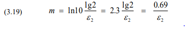
Similarly, a strict mathematical relation can be determined for the Swedish-Finnish e2-approach (Eq. 3.6), as described in Eq. 3.19.

The Janbu method of treating the intermediate soils (sandy silt, silty sand, and sand) is “extra” to the Cc-e0 method and the elastic method (Eqs. 3.12 and 3.13).

It is not possible to express the relative degree of compressibility using the Cc-e0 approach. That is, a specific Cc-value cannot be referred to as representing a high compressibility or medium compressibility, etc., without also coupling it with the e0-value and few can correlate to two numbers simultaneously. The following couple of examples will demonstrate the advantage of the Janbu modulus number approach as opposed to the conventional Cc /e0 approach.

Figure 3.3 shows results from oedometer tests on an overconsolidated Texas Gulf Clay (Beaumont clay), with void ratios ranging from about 0.4 through 1.2 (Endley et al. 1996). Figure 3.3A presents a range of Cc-values, which imply that the compressibility expressed as increased Cc-value, would be increasing with depth (the associated values of voids ratio, e, are not shown . However, Fig. 3.3B, which shows the Cc-e0-values converted to Janbu modulus numbers, demonstrates that there is no such trend with depth. The modulus numbers range—from about 10 through almost 40—is quite wide, going from high through low compressibility.

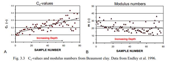
Figure 3.4 presents results from oedometer tests on a normally consolidated to slightly overconsolidated silty clay outside Vancouver, BC with void ratios ranging from about 0.8 through 1.4. The relative range between the smallest and largest Cc-value (a factor of 2) suggests a somewhat wider range of compressibility than the actual, represented by the modulus number where the relative range between the smallest and largest value is a factor of 1.3. The average modulus number is approximately 10, which is the upper boundary of a very compressible soil.

The Janbu method is widely used internationally and by several North American engineering companies and engineers. However, many others are yet reluctant to use the Janbu approach, despite its obvious advantages over the conventional Cc /e0 method. The approach has been available for more than twenty years in the second and third editions of the broadly used Canadian Foundation Engineering Manual, CFEM (1985; 1992). (Regrettably, by accident or other, the committee revising the CFEM for the fourth Edition published in 2006 omitted to keep the Janbu approach in the Manual). Moreover, the Janbu modulus number has important application for assessing liquefaction risk and soil densification as described in Section 2, Clauses 12.8,4 and 2.12.8.5.

Those not fully convinced by the previous examples, should reflect on the results shown in Fig. 3.5 and 3.6. Figure 3.5A shows a fairly typical array of Cc-values ranging from about 0.3 through 0.9, implying a rather randomly varying compressibility. However, when coupled with the associated e0-values, admittedly judiciously selected, as shown in Fig. 3.5B, the different picture evolves: the compressibility is constant for the Cc-values. Figure 3.6A shows a set of constant Cc-values, that is, they imply a constant compressibility. Similarly, however, when coupled with their associated e0-values, again admittedly judiciously selected, as shown in Fig. 3.6B, the different picture evolves: the compressibility is highly variable despite the constant Cc-values.

Engineers working in a well-known area where the soils have a familiar range of water contents and void ratios well-known to those engineers, can work well only classifying compressibility from Cc-values. However, when encountering foundation problems in different geologies, a good advice is to start using the modulus number as the measure of and reference to soil compressibility.