Basic principles of traffic demand analysis

If transport planners wish to modify a highway network either by constructing a new roadway or by instituting a programme of traffic management improvements, any justification for their proposal will require them to be able to formulate some forecast of future traffic volumes along the critical links. Particularly in the case of the construction of a new roadway, knowledge of the traffic volumes along a given link enables the equivalent number of standard axle loadings over its lifespan to be estimated, leading directly to the design of an allowable pavement thickness, and provides the basis for an appropriate geometric design for the road, leading to the selection of a sufficient number of standard width lanes in each direction to provide the desired level of service to the driver. Highway demand analysis thus endeavours to explain travel behaviour within the area under scrutiny, and, on the basis of this understanding, to predict the demand for the highway project or system of highway services proposed.

 The prediction of highway demand requires a unit of measurement for travel behaviour to be defined. This unit is termed a trip and involves movement from a single origin to a single destination. The parameters utilised to detail the nature and extent of a given trip are as follows:

·         Purpose

·         Time of departure and arrival

·         Mode employed

·         Distance of origin from destination

·         Route travelled.

Within highway demand analysis, the justification for a trip is founded in economics and is based on what is termed the utility derived from a trip. An individual will only make a trip if it makes economic sense to do so, i.e. the economic benefit or utility of making a trip is greater than the benefit accrued by not travelling, otherwise it makes sense to stay at home as travelling results in no economic benefit to the individual concerned. Utility defines the ‘usefulness’ in economic terms of a given activity. Where two possible trips are open to an individual, the one with the greatest utility will be undertaken. The utility of any trip usually results from the activity that takes place at its destination. For example, for workers travelling from the suburbs into the city centre by car, the basic utility of that trip is the economic activity that it makes possible, i.e. the job done by the traveller for which he or she gets paid. One must therefore assume that the payment received by a given worker exceeds the cost of making the trip (termed disutility), otherwise it would have no utility or economic basis. The ‘cost’ need not necessarily be in money terms, but can also be the time taken or lost by the traveller while making the journey. If an individual can travel to their place of work in more than one way, say for example by either car or bus, they will use the mode of travel that costs the least amount, as this will allow them to maximise the net utility derived from the trip to their destination. (Net utility is obtained by subtracting the cost of the trip from the utility generated by the economic activity performed at the traveller’s destination.)

Demand modelling

Demand modelling requires that all parameters determining the level of activity within a highway network must first be identified and then quantified in order that the results output from the model has an acceptable level of accuracy. One of the complicating factors in the modelling process is that, for a given trip emanating from a particular location, once a purpose has been established for making it, there are an enormous number of decisions relating to that trip, all of which must be considered and acted on simultaneously within the model. These can be classified as:

·         Temporal decisions – once the decision has been made to make the journey, it still remains to be decided when to travel

·         Decisions on chosen journey destination – a specific destination must be selected for the trip, e.g. a place of work, a shopping district or a school

·         Modal decisions – relate to what mode of transport the traveller intends to use, be it car, bus, train or slower modes such as cycling/walking

·         Spatial decisions – focus on the actual physical route taken from origin to final destination. The choice between different potential routes is made on the basis of which has the shorter travel time.

If the modelling process is to avoid becoming too cumbersome, simplifications to the complex decision-making processes within it must be imposed. Within a basic highway model, the process of simplification can take the form of two stages:

(1) Stratification of trips by purpose and time of day

(2) Use of separate models in series for estimating the number of trips made from a given geographical area under examination, the origin and destination of each, the mode of travel used and the route selected.

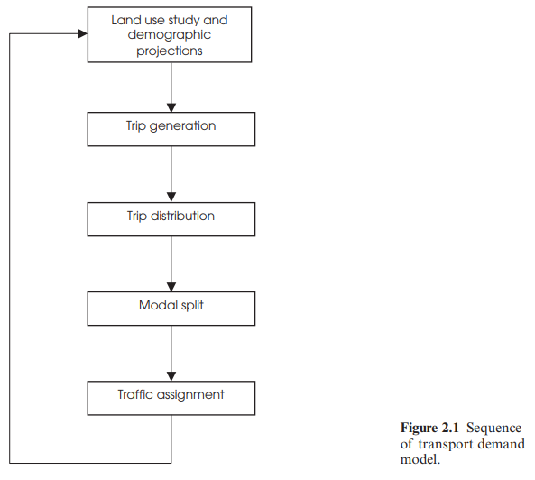
Stratification entails modelling the network in question for a specific time of the day, most often the morning peak hour but also, possibly, some critical off-peak period, with trip purpose being stratified into work and non-work. For example, the modeller may structure the choice sequence where, in the first instance, all work-related trips are modelled during the morning peak hour. (Alternatively, it may be more appropriate to model all non-work trips at some designated time period during the middle of the day.) Four distinct traffic models are then used sequentially, using the data obtained from the stratified grouping under scrutiny, in order to predict the movement of specific segments of the area’s population at a specific time of day. The models are described briefly as:

·         The trip generation model, estimating the number of trips made to and from a given segment of the study area

·         The trip distribution model, estimating the origin and destination of each trip

·         The modal choice model, estimating the form of travel chosen for each trip

·         The route assignment model, predicting the route selected for each trip.

Used in series, these four constitute what can be described as the basic travel demand model. This sequential structure of traveller decisions constitutes a considerable simplification of the actual decision process where all decisions related to the trip in question are considered simultaneously, and it provides a sequence of mathematical models of travel behaviour capable of meaningfully forecasting traffic demand.

An overall model of this type may also require information relating to the prediction of future land uses within the study area, along with projections of the socio-economic profile of the inhabitants, to be input at the start of the modelling process. This evaluation may take place within a land use study.

Figure 2.1 illustrates the sequence of a typical transport demand model.

At the outset, the study area is divided into a number of geographical segments or zones. The average set of travel characteristics for each zone is then determined, base on factors such as the population of the zone in question. This grouping removes the need to measure each inhabitant’s utility for travel, a task which would in any case from the modeller’s perspective be virtually impossible to achieve.

The ability of the model to predict future travel demand is based on the assumption that future travel patterns will resemble those of the past. Thus the model is initially constructed in order to predict, to some reasonable degree of accuracy, present travel behaviour within the study area under scrutiny. Information on present travel behaviour within the area is analysed to determine meaningful regression coefficients for the independent variables that will predict the dependent variable under examination. This process of calibration will generate an equation where, for example, the existing population of a zone, multiplied by the appropriate coefficient, added to the average number of workers at present per household multiplied by its coefficient, will provide the number of

work trips currently originating from the zone in question. Once the modeller is satisfied that the set of values generated by the process is realistic, the calibration stage can be completed and the prediction of trips originating from the zone in question at some point in the future can be estimated by changing the values of the independent variables based on future estimates from experts.