Trip production

Assume a study area is divided into seven zones (A, B, C, D, E, F, G) as indicated in Fig. 2.3. Transport planners wish to estimate the volume of car traffic for each of the links within the network for ten years into the future (termed the design year).

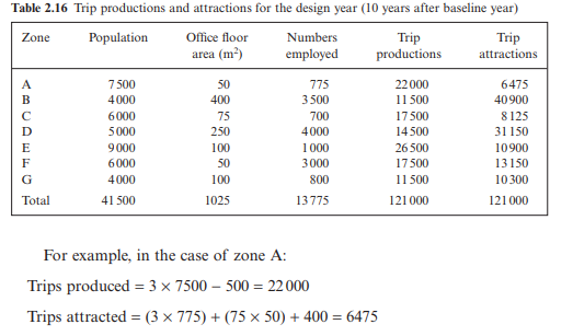
Using land use data compiled from the baseline year on the trips attracted to and generated by each zone, together with information on the three main trip generation factors for each of the seven zones:

·         Population (trip productions)

·         Retail floor area (trip attractions)

·         Employment levels (trip attractions)

linear regression analysis yields the following zone-based equations for the two relevant dependent variables (zonal trip productions and zonal trip attractions) as follows:

Table 2.16 gives zonal trip generation factors for the design year, together with the trip productions and attractions estimated from these factors using Equations 2.17 and 2.18

Trip distribution

 In order to compile the trip distribution matrix, the impedance term relating to the resistance to travel between each pair of zones must be established. In this case, the travel time is taken as a measure of the impedance and the zone-tozone times are given in Table 2.17.

Using a gravity model with the deterrence function in the following form between zone i and zone j:

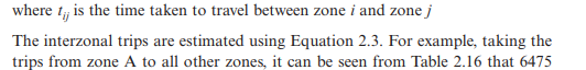
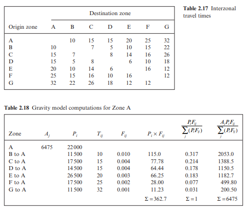
trips were attracted to zone A. Equation 2.3 is used to estimate what proportion of this total amount sets out from each of the other six zones, based on the relative number of trips produced by each of the six zones and the time taken to travel from each to zone A. These computations are given in Table 2.18.

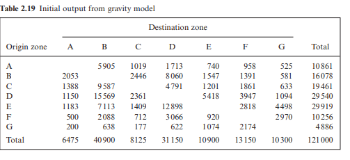
When an identical set of calculations are done for the other six zones using the gravity model, the initial trip matrix shown in Table 2.19 is obtained.

It can be seen from Table 2.19 that, while each individual column sums to give the correct number of trips attracted for each of the seven zones, each individual row does not sum to give the correct number of trips produced by each. (It should be noted that the overall number of productions and attractions are equal at the correct value of 121 000.)

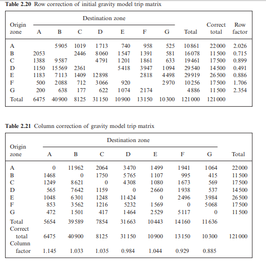
In order to produce a final matrix where both rows and columns sum to their correct values, a remedial procedure must be undertaken, termed the row column factor technique. It is a two-step process. First, each row sum is corrected by a factor that gives the zone in question its correct sum total (Table 2.20).

Second, because the column sums no longer give their correct summation, these are now multiplied by a factor which returns them to their correct individual totals (Table 2.21).

This repetitive process is continued until a final matrix is obtained where the production and attraction value for each zone is very close to the correct row and column totals (Table 2.22)

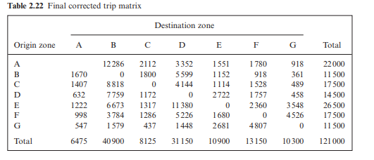
(Note, if Equation 2.2 is used within the trip distribution process, the rows sum correctly whereas the columns do not. In this situation the row-column factor method is again used but the two-stage process is reversed as a correction is first applied to the column totals and then to the new row totals.)