A second method to determine the value of the coefficient of consolidation is to use only the results of a consolidation test for small values of time, and to use the fact that in the beginning of the process its progress is proportional to the square root of time. In this method the measurement data are plotted against √ t, see Figure 18.2. The basic formula is, see (16.22),
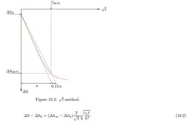
In principle the value of the coefficient of consolidation cv could be determined from the slope of the straight line in the figure, but this again requires the value of the initial deformation and the final deformation, as these appear in the formule (18.2). The value of the initial deformation ∆h0 can be determined from the intersection point of the straight tangent to the curve with the axis √ t = 0. The final deformation ∆h∞, however, can not be obtained directly from the data. In order to circumvent this difficulty Taylor has suggested to use the result following from the theoretical curve and its approximation that for U = 0.90, i.e. for 90 % of the consolidation, the value of √ t according to the exact solution is 15 % larger that the value given by the approximate formula (18.2). The exact formula (16.11) gives that U = 0.90 if cvt/h2 = 0.8481, and the approximate formula (18.2) gives that U = 0.90 for cvt/h2 = 0.6362. The ratio of these two values is 1.333, which is the square of 1.154. If in Figure 18.2 a straight line is plotted at a slope that is 15 % smaller than the tangent to the measurement data for small values of time, this line should intersect the measured curve in the point for which U = 0.90. The corresponding value of the time parameter cvt/h2 is 0.848, and therefore the consolidation coefficient can be determined as

If the theory of consolidation were an exact description of the real behaviour of soils, the two methods described above should lead to exactly the same value for the coefficient of consolidation cv. Usually this appears to be not the case, with errors of the order of magnitude up to 10 or 20 %. This indicates that the measurement data may be imprecise, especially when the deformations are very small, or that the theory is less than perfect. Perhaps the weakest point in the theory is the assumption of a linear relation between stress and strain.
Determination of mv and k
In both of the two methods, the log(t)-method and the √ t-method, the procedure includes a value for the final consolidation settlement of the sample, even though it is realized that the deformations may continue beyond that value. In the log(t)-method this final value forms part of the analysis, in the √ t-method the final value of the deformation can be determined by adding 10 % to the difference of the level of 90 % consolidation and the initial deformation,

In general the final deformation is

so that the value of the compressibility mv follows from

Because the coefficient of consolidation cv has been determined before, it follows that the permeability k can be determined as

The determination of the permeability k and the compressibility mv may be theoretically unique, but due to theoretical approximations and inaccuracies in the measurement data the accuracy in the actual values may not be very large.