As an example the flow under a structure will be considered, see Figure10.2. In this case a sluice has been constructed into the soil. It is assumed that the water level on the left side of the sluice is a distance H higher than the water on the right side. At a certain depth the permeable soil rests on an impermeable layer. To restrict the flow under the sluice a sheet pile wall has been installed on the upstream side of the sluice bottom.

The flow net for a case like this can be determined iteratively. The best procedure is by sketching a small number of stream lines, say 2 or 3, following an imaginary water particle from the upstream boundary to the downstream boundary. These stream lines of course must follow the direction of the constraining boundaries at the top and the bottom of the flow field. The knowledge that the stream lines must everywhere be perpendicular to the potential lines can be used by drawing the stream lines perpendicular to the horizontal potential lines to the left and

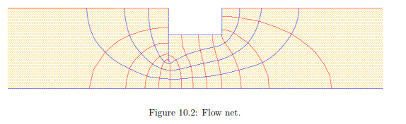
to the right of the sluice. After completion of a tentative set of stream lines, the potential lines can be sketched, taking care that they must be perpendicular to the stream lines. In this stage the distance between the potential lines should be tried to be taken equal to the distance between the stream lines. In the first trial this will not be successful, at least not everywhere, which means that the original set of stream lines must be modified. This then must be done, perhaps using a new sheet of transparent paper superimposed onto the first sketch. The stream lines can then be taken such that a better approximation of squares is obtained.

The entire process must be repeated a few times, until finally a satisfactory system of squares is obtained, see Figure 10.2. Near the corners in the boundaries some special ”squares” may be obtained, sometimes having 5 sides. This must be accepted, because the boundary imposes the bend in the boundary. In the case of Figure 10.2 at the right end of the net one half of a square is left. It turns out that there are 12.5 intervals between potential lines, which means that the interval between two potential lines is

Because the flow net consists of squares it follows that ∆Ψ = ∆Φ, so that

Because there appear to be 4 stream bands, the total discharge now is

in which B is the width perpendicular to the plane of the figure. The value of the discharge Q must be independent of the number of stream lines that has been chosen, of course. This is indeed the case, as can be verified by repeating the process with 4 interior stream lines rather than  3. It will then be found that the number of potential intervals will be larger, about in the ratio 5 to 4. The ratio of the number of squares in the direction of flow to the number of squares in the direction perpendicular to the flow remains (approximately) constant.

From the completed flow net the groundwater head in every point of the field can be determined. For instance, it can be observed that between the point at the extreme left below the bottom of the sluice and the exit point at the right, about 6 squares can be counted (5 squares and two halves). This means that the groundwater head in that point is

if the head is measured with respect to the water level on the right side.

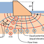
The pore water pressure can be derived if the head is known, as well as the elevation, because h = z + p/γw. The evaluation of the water pressure may be of importance for the structural engineer designing the concrete floor, and for the geotechnical engineer who wishes to know the effective stresses, so that the deformations of the soil can be calculated. From the flow net the force on the particles can also be determined (the seepage force). According to equation (6.16) the seepage force is

In the case illustrated in Figure 10.2 it can be observed that at the right hand exit, next to the structure, in the last (half) square ∆h = −H/(2 × 12.5) and ∆z = 0.3 d, if d is the depth of the structure into the ground. Then, approximately, ∂h/∂z = −0.133 H/d, so that jz = 0.133γw H/d. This is a positive quantity, indicating that the force acts in upward direction, as might be expected. The particles at the soil surface are also acted upon by gravity, which leads to a volume force of magnitude −(γs − γw), negative because it is acting in downward direction. It seems tempting to conclude that there is no danger of erosion of the soil particles if the upward force is smaller than the downward force. This would mean, assuming that γs/γw = 2, so that (γs − γw)/γw = 1, that the critical value of H/d would be about 7.5. Only if the value of H/d would be larger than 7.5 erosion of the soil would occur, with the possible loss of stability of the floor foundation at the right hand side.

In reality the danger may be much larger. If the soil is not completely homogeneous, the gradient ∂h/∂z at the downstream exit may be much larger than the value calculated here. This will be the case if the soil at the downstream side is less permeable than the average. In that case a pressure may build up below the impermeable layer, and the situation may be much more dangerous. On the basis of continuity one might say, very roughly, that the local gradient will vary inversely proportional to the value of the hydraulic conductivity, because k1i1 = k2i2. This means that locally the gradient may be much larger than the average value that will be calculated on the basis of a homogeneous average value of the permeability. Locally soil may be eroded, which will then attract more water, and this may lead to further erosion. The phenomenon is called piping, because a pipe may be formed, just below the structure. Piping is especially dangerous if a structure is built directly on the soil surface. If the structure of Figure 10.2 were built on the soil surface, and not into it, the velocities at the downstream side would be even larger (the squares would be very small), with a greater risk of piping. Prescribing a safe value for the gradient is not so simple. For that reason large safety factors are often used. In the case of vertical outflow, as in Figure 10.2, a safety factor 2, or even larger, is recommended. In cases with horizontal outflow the safety factor must be taken much larger, because in that case there is no gravity to oppose erosion. In many cases piping has been observed, even though the maximum gradient was only about 0.1, assuming homogeneous conditions. Technical solutions are reasonably simple, although they may be costly. A possible solution is that on the upstream side, or near the upstream side, the resistance to flow is enlarged, for instance by putting a blanket of clay on top of the soil, or into it. Another class of solutions is to apply a drainage at the downstream side, for instance by the installation of a gravel pack near the expected outflow boundary. In the case of Figure 10.2 a perfect solution would be to make the sheet pile wall longer, so that it reaches into the impermable layer. A large dam built upon a permeable soil should be protected by an impermeable core or sheet pile wall, and a drain at the downstream side. The large costs of these measures are easily justified when compared to the cost of loosing the dam.