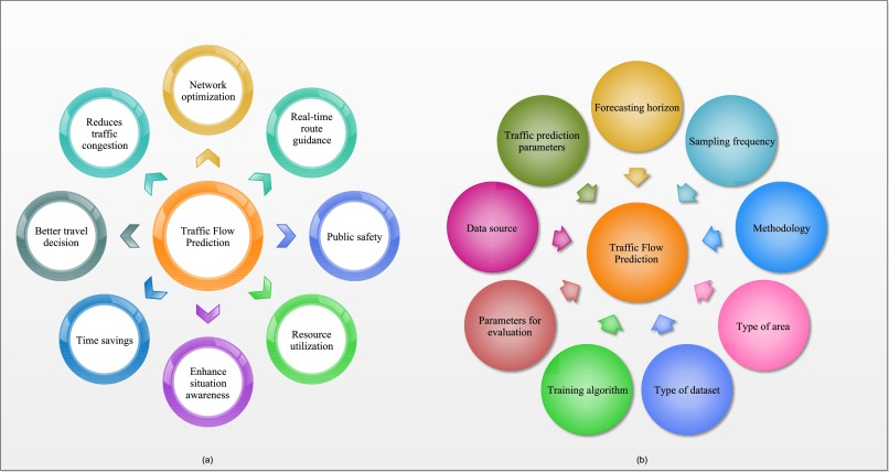
In this paper, different artificial neural network (ANN) models for predicting the hourly traffic flow in Second Tolled Bridge of Bosphorus in Turkey is performed. Second Bosphorus Bridge has an important role in urban traffic networks of Istanbul. The prediction of the traffic flow data is a vital requirement for advanced traffic management and traffic information systems, which aim to influence the traveler behaviors, reducing the traffic congestion, improving the mobility and enhancing the air quality. Detecting the trends and patterns in transportation data is a popular area of research in the business world to support the decision-making processes. The primary means of detecting trends and patterns has involved statistical methods such as clustering and regression analysis most of which use linear models. The goal is to predict a future value of data by using the past data set. On the other hand, non-linear approaches offer more powerful models, since they give more possibilities in the choice of the input-output relation.
ANNs approaches have been applied to a large number of problems because of their nonlinear system modeling capability by learning ability using collected data. They offer highly parallel, adaptive models that can be trained by the experience. During the last decade, ANN has been applied widely to prediction of the traffic data.
We compared the generalization performance of the different ANN models such as Multi Layer Perceptron (MLP), Radial Basis Function Network (RBF), Elman Recurrent Neural Networks (ERNN) and Non-linear Auto Regressive and eXogenous input (NARX) type.
Traffic flow prediction
Detecting the trends and patterns in transportation data is a popular area of research in the business world to support the decision-making processes (Topuz, 2007). According to the theory, the traffic flow forecasting research can be divided into two types. One type is determined based on the mathematical model and second type is knowledge-based intelligent model of forecasting methods. Short-term traffic flow prediction is more influenced by the stochastic interferential factors than the long-term one, the uncertainty is greater and the disciplinarian laws are less obvious. Thus using the short-term traffic prediction models based on the classical mathematical methods, the precision of forecast cannot satisfactorily meet the demand of real-time traffic control systems (Su & YU, 2007).
Source: Urban Transport and Hybrid Vehicles, Book edited by: Seref Soylu,
ISBN 978-953-307-100-8, pp. 192, September 2010, Sciyo, Croatia, downloaded from SCIYO.COM
Because the traffic system is a complex and variable system that involves a great deal of people, the traffic flow state has high randomness and uncertainty. The traditional traffic flow forecast methods such as Kalman filter, Moving Average (MA), Autoregressive Integrated Moving Average (ARIMA) and etc had been unable to satisfy the demand of the forecast precision that was increasing in practice (CHEN & MA, 2009)
On the other hand, artificial neural networks (ANNs) have been applied to a large number of problems because of their non-linear system modeling capacity by learning ability using collected data. During the last decade ANNs have been applied widely to prediction of the traffic data (SADEK, 2007). Different ANN approach such as MLP (Smith &. Demetsky, 1994), RBF (Celikoglu & Cigizoglu, 2006), ERNN (Li & Lu, 2009), Neuro-Genetic (Abdulhai et al. 2002) have been used to predict the traffic follow.
Such a prediction study including the NARX type ANN has been completed in this paper, to compare the effectiveness of different ANN approach.
Artificial Neural Network (ANN)
ANNs are designed to mimic the characteristics of the biological neurons in the human brain and nervous system. Given a sample vectors, ANNs is able to map the relationship between input and output; they “learn” this relationship, and store it into their parameters.. The training algorithm adjusts the connection weights (synapses) iteratively learning typically occurs through the training. When the network is adequately trained, it is able to generalize relevant output for a set of input data. They have been applied to a large number of problems because of their non-linear system modeling capacity.
Multi Layer Perceptron (MLP)
There are different types of ANN although the most commonly used architecture of ANN is the multilayer perceptron (MLP). MLP has been extensively used in many transportation applications due to its simplicity and ability to perform nonlinear pattern classification and function approximation. Therefore, it is considered the most commonly implemented network topology by many researchers (Transportation Research Board 2007).
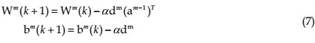
MLP means a feedforward network with one or more layers of nodes between the input and output nodes and it is capable of approximating arbitrary functions. Two important characteristics of the MLP are: its nonlinear processing elements (activation function) which have a nonlinearity and their massive interconnectivity (weights).Typical MLP network is arranged in layers of neurons, where each neuron in a layer computes the sum of its inputs and passes this sum through an activation function (f). For this context designed MLP network is shown in figure 1.
The MLP network is trained with back-propagation, the first step is propagating the inputs towards the forward layers through the network. For a three-layer feed-forward network, training process is initiated from the input layer (Hagan 1996).
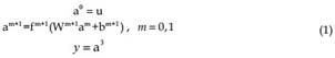
Where, y is output vector, u is input vector, f (.) is the activation function, W is weighting coefficients matrices, b is bias factor vector and m is the layer index. These matrices defined as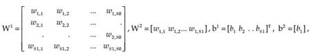
Here S0 and S1 are size of network input and hidden layer
In this study, sigmoid tangent activation functions are used in the hidden layer and linear activation function is used in the output layer respectively. These functions are defined as follows;
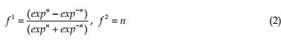
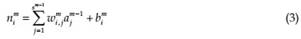
The total network output is ;
Second step is propagating the sensibilities (d) from the last layer to the first layer through the network: d ,d ,d3 2 1 . The error (e) calculated for output neurons is propagated to the backward through the weighting factors of the network. It can be expressed in matrix form as follows: 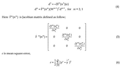 Where γ is the sample in dimension q.The last step in back-propagation is updating the weighting coefficients. The state of the network always changes in such a way that the output follows the error curve of the network towards down.
where α represents the training rate, k represents the epoch number. By the algorithmic approach known as gradient descent algorithm using approximate steepest descent rule, the error is decreased repeatedly
Fig. 1. Designed MLP Network Schematic Diagram.
Elman Recurrent Neural Networks (ERNN)
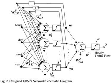
ERNN is also known partially recurrent neural network which is subclass of recurrent networks. It is MLP network augmented with additional context layers (W0), storing output values (y), of one of the layers delayed (z-1) by one-step and used for activating this other layer in the next time (t) step. The self-connections of the context nodes make it also sensitive to the history of input data, which is very useful in dynamic system modeling (Elman, 1990).

While ERNN use identical training algorithm as MLP, context layer weight (W0) is not updated as in equation 8. Schematic diagram of designed ERNN network is given in figure 2.The ERNN network can be trained with any learning algorithm that is applicable to MLP such as backpropagation that is given above.
Radial Basis Function Network (RBF)
RBF network has a feed-forward structure consisting of two layers, nonlinear hidden layer and linear output which is given in figure in 3. RBF networks are being used for function approximation, pattern recognition, and time series prediction problems. Their simple structure enables learning in stages, and gives a reduction in the training time.
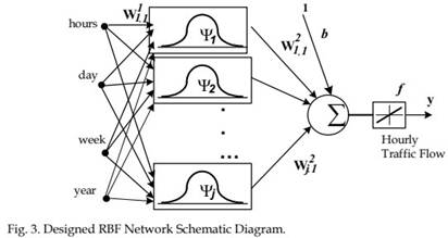
The proposed model uses Gaussian kernel (Ψ) as the hidden layer activation function. The output layer implements a linear combiner of the basis function responses defined as; (Haykin, 1994)
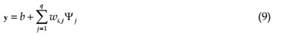
Where, q is the sample size, Ψj is response of the jth hidden neuron described as;
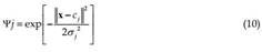
Where, cj is Gaussian function center value, and σj is its variance.
RBF network training has two-stage procedure. In the first stage, the input data set is used to determine the center locations (cj) using unsupervised clustering algorithm such as the Kmeans algorithm and choose the radii (σj) by the k-nearest neighbor rule. The second step is to update the weights (W)of the output layer, while keeping the (cj) and (σj) are fixed.
Non-linear Auto Regressive and eXogenous Input type ANN (NARX)
A simple way to introduce dynamics into MLP network consists of using an input vector composed of past values of the system inputs and outputs. This the way by which the MLP can be interpreted as a NARX model of the system. This way of introducing dynamics into a static network has the advantage of being simple to implement. To deduce the dynamic model of realized system, NARX type ANN model can be represented as follows (Maria & Barreto, 2008);

where y(k+1) is model predicted output, fANN is a non-linear function describing the system behavior, u(k), y(k), ε(k)are input, output and approximation error vectors at the time instances k, n and m the orders of y(k) and u(k) respectively. Order of the process can be estimated from experience. Modeling by ANN relies on the consideration of an approximate function of fANN. Approximate dynamic model is constructed by adjusting a set of connection weight (W) and biases (b) via training function defined as MLP network. The NARX network, it can be carried out in one out of two modes:
Series-Parallel (SP) Mode: In this case, the output’s regressor is formed only by actual values of the system’s output defined as;

Figure 4 shows the topology of one-hidden-layer NARX network when trained in the SPmode.
Parallel (P) Mode:In this case, estimated outputs are fed back and included in the output’s regressor defined as follows;

While NARX-SP type network is used in the training phase, NARX -P type network isused in the testing phase, which is given in figure 5.
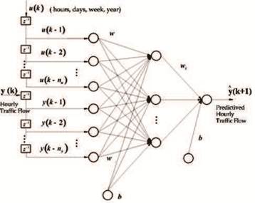
Fig. 4. Architecture of the NARX network during training in the SP-mode
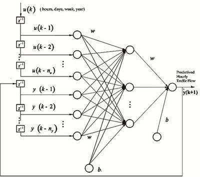
Fig. 5. Architecture of the NARX network during testing in the P-mode.
Designing process
ANN designing process involves four steps. These are gathering the traffic data, selecting the ANN architecture, training the network, and testing the network. In the training, four input variables have been used. These are, hours of the day: 0-23; days of the month: 1-30; days of the week: 1-7; and years: 2001-2003. Selecting the daily traffic demands as distinct variables both for days of the month and days of the week are mandatory situation, because of the weekly and monthly variance of the daily traffic demands. In the training phase, the target variables have been used as 2160 data related to the volumes, or hourly passing number of the vehicles (demand) of 4th months (April) of the years 2001-2003. In the testing phase, 720 data related to the hourly demand of 4th month (April) of the year 2004, have been used to compare the actual and neural output of the system performance.
Gathering the Traffic Data: Data recorded by the tolls has been used for training, testing and analysis. Only 2880 number of traffic demand data related to the hours of the days of 4th months of the years 2001-2004 has been taken into consideration (Transportation Survey 2004). Selecting the Best Network Architecture: The number of hidden layer and neurons in the hidden layer(s) play very important roles for ANNs and choice of these numbers depends on the application. Influenced by theoretical works proved that single hidden layer is sufficient for ANNs to approximate any complex nonlinear function with any desired accuracy. In addition, determining the optimal number of hidden neurons is still a question to deal with. Although there is no theoretical basis for selecting these parameters, a few systematic approaches are also reported but the most common way of determining the number of hidden neurons is still trial and error approach. The number of input nodes that depend on the number of the time lags is also very important for the performance of the NARX type ANN model. The value of the time lags has to be determined by trial and error effort. Radius of the center point in nonlinear activation function is great effect the performance of the RBF network. Therefore, in addition to hidden layer neuron number, radiuses of the center point in neurons are also determined.
Training and testing the network: Designed MLP, ERNN and NARX network are trained with Levenberg-Marquardt backpropagation learning algorithms, which described in section 3. MATLAB with Neural network toolbox is used for all ANN application (Demuth & Beale 2002).
The optimum learning, η and the momentum, α, rates are determined after trials observing the RMSE and R obtained at the end of the testing stage. When a smaller η is selected, the changes to the synaptic weights (W) in the network had been smaller. The momentum rates α prevented the learning process from terminating in a local minimum of the error surface. It is seen that η and α should be decreased if the number of the input and output layers are increased. On the other hand, the iteration number increases by decreasing η and α value. Once trained, the network can be used for predicting (test phase) the output for any input vector from the input space. This is called the “generalization property” of the network. To show this property of trained networks, the same experiment is done with testing data set that are not involved in training data set. It is also used the early stopping strategy (validation phase) to improve the generalization properties of designed network. In this strategy, the validation data set is used and the error on the validation set is monitored during the training process. The validation error normally decreases during the initial phase of training. However, when the network begins to overfit the data, the error on the validation set typically begins to rise. When the validation error increases for a specified number of iterations, which we choose 10, the training process is stopped. Root mean square error (RMSE) values and correlations coefficients (R) are selected to compare the performance of designed network, which is defined as follows;
Features may be correlated, that is, a change in one feature Y is associated with a similar change in another feature Yˆ . A correlation coefficient can be calculated as;
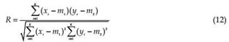
Here m1 is the mean value of all the values xi of feature Y, and m2 is the mean of all yi values of the Yˆ feature. The correlation coefficient assumes values in the interval [-1,1]. When R= 1 there is a strong negative correlation between Y and Yˆ , when R=1 there is a strong positive correlation, and when R=0 there is no correlation at all. Root mean squared error is also defined as follows;

Where q is sample size, yi, yˆi are network output and predicted output respectively.
Experiments and results
In this section, firstly the performance of all MLP, ERNN, RBF and NARX type ANN model are investigated. Then scattering diagram and traffic flow graphics are drawn for the best ANNs models.
MLP network experiments
As a mentioned above, the performance of MLP network is highly dependent on the hidden layer neuron number. Therefore, performances of MLP network is tested using 5, 10,15,25,50 and 100 neurons in the hidden layer. End of the training and testing procedure s obtained correlations coefficients (R) and MSE values are given in table 1.
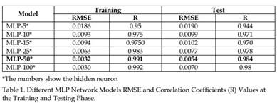
It could be easily figure out in this table that, MLP-50 network shows the best generalization performance. It is also realized that to use more than 50 neurons in the hidden layer are not increase the generalization ability of designed networks. The best MLP network model scattering diagram is shown in figure 6.
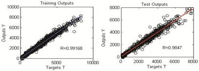
Fig. 6. MLP-50 Network Model Scattering Diagrams for Train and Test Output.
To show the obtained results, for only last week’s predicted values with real traffic flow are given in figure 7. These figures with scattering diagrams show us that prediction errors are small enough to be accepted
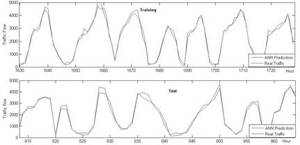
Fig. 7. The Best MLP Network Model Traffic Flow Graphics at the Train and Testing Phase.
ERN network experiments
The performance of ERNN is also dependent on the hidden layer neuron number. Hence, performances of ERNN is tested using 5, 10,15,25,50,100 neurons and obtained correlations coefficients (R) and MSE values are given in table 2. It could be easily figure out in this table that, ERNN -10 network shows the best generalization performance. The best ERNN model scattering diagram is shown in figure 8. Achieved the best ERNN results, with real traffic flow are given in figure 7.
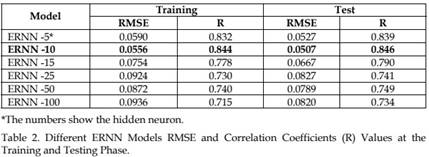
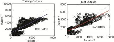
Fig. 8. ERNN -10 Network Scattering Diagrams for Train and Test Output.
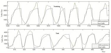
Fig. 9. The Best ERNN Model Traffic Flow Graphics at the Train and Testing Phase
RBF network experiments
Because of the performance of RBF network is depending on the radius of the center points and hidden layer neuron number, different RBF network models are tested. Obtained correlations coefficients (R) and MSE values are given in table 3. It could be easily figure out in this table that, RBF N250/S2 network shows the best generalization performance. The best RBF network model scattering diagram is shown in figure 10. Related traffic flow graphics on the test and training data is also given in figure 11.
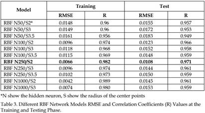
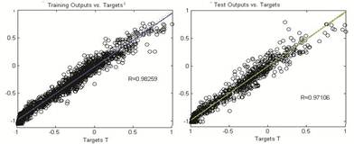
Fig. 10. RBF N250/S2 -10 Network Scattering Diagrams for Train and Test Output.
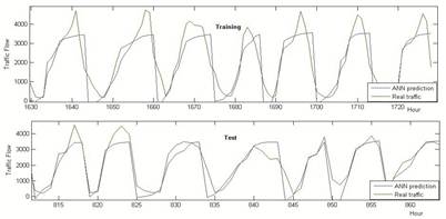
Fig. 11. Best RBF Network Model Traffic Flow Graphics at the Train and Testing Phase
NARX network experiments
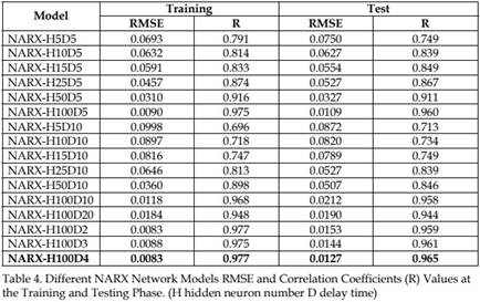
The number of input nodes to the NARX type ANN model is dependent on the number of the time lags that is determined by the analysis of the auto-correlation function belonging to examined time series data set. Four time lags are found sufficient, hence; the input layer consisted of four nodes. Because the second step is largely a trial-and-error process and experiments involving neural networks with more than 4 input nodes and more than 100 neurons in the hidden layer didn’t show any improvement in prediction accuracy. Obtained correlations coefficients (R) and MSE values are given in table 4, The best NARX network model scattering diagram is shown in figure 12.
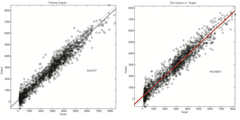
Fig. 12. NARX-H100D4 Network Scattering Diagrams for Train and Test.
Achieved predicted values with real traffic flow are given in figure13. These figures with scattering diagrams show us that prediction errors are small enough to be accepted.
Conclusion
In this paper, different ANN models have predicted daily traffic demand in Second Tolled Bridge of Bosphorus, which has an important role in urban traffic networks of Istanbul. To find the best-predicted model feed forward type (MLP, RBF), recurrent type (ERNN) and NARX type ANNs are used. Previously every model parameters are investigated for each network type. In this stage, root mean square errors (RMSE) and correlation coefficient (R) values are used as a performance criterion.
Concerning neural networks that are created and simulated there have been excluded the below conclusions:
• The most efficient training algorithm proved to be the Levenberg-Marquardt
Backpropagation, as it surpassed the others not only in quality of results but also in speed.
• For the MLP, ERNN and NARX type network, the best type of normalization proved to be the one in region -1 -1 in combination with sigmoid tangent activation function in the hidden layer nodes. For the RBF network, the best radius of the center points is found 2. For a NARX network, suitable choice of input delay is 4
• The number of nodes used in the hidden layer depends from the type and the complexity of the time series, and from the number of inputs.
• The results have shown that feed forward type network models have advantages over recurrent type network.
• It is also concluded that, many other transportation data prediction studies can be implemented easily and successfully by using the different ANN architectures.