The current energy scenery is dominated by fossil fuels, especially oil. This dependency is turning critical due to the reducing reserves, uncertain oil resources, and political and economical ramifications of a concentration of fossil fuel reserves in a limited number of regions. The transportation sector is especially affected by this situation and needs to develop new energy vectors and systems to reduce the oil dependency whilst attending to environmental issues. Therefore, vehicle manufacturers are turning to hybrid and electric vehicles. Hybrid vehicles combine an internal combustion engine (ICE) with energy storage systems, which allows reducing the installed power of the ICE, and consequently the fuel consumption and pollutant emissions. With this power train, the user is capable of driving in a pure electric mode, through the energy storage system (normally batteries), or in a hybrid mode with both ICE and storage for more challenging driving cycles.
Electric vehicles are especially interesting due to the exclusion of the ICE, which reduces to zero the emissions, and presents a higher efficiency of the power train and environmentally friendly operation. However, even if these reasons are activating its interest, there are several drawbacks which should be solved before reaching a mass production scale. Some of these issues include the development of energy technologies able to guarantee an adequate vehicle range, attractive power ratings and safe, simple and fast recharge.
Nowadays there is no electric energy storage technology which can exhibit both high energy and power densities, necessary to meet range and accelerating requirements. Therefore, there is an intensive research to develop new materials for electrochemical energy devices and to hybridize electrochemical energy systems to reach the necessary power and energy specifications. The most popular technologies are Ni-Mh and Li-based batteries, which present higher energy densities than classic Pb-acid batteries. However, these technologies cannot achieve the range obtained with fossil fuels. Therefore, other energy systems, such as fuel cells or flow batteries are being studied as part of a hybrid electric vehicle power train.
Finally, this energy system research should be done taking into account the particular situation of transportation, where the weight, volume and cost of the systems included are relevant for a successful and massive use of the electric vehicle. To carry out this research in the final application stage of electrochemical systems, it is necessary to be able to test, model and simulate this system in real operating conditions.
Source: Urban Transport and Hybrid Vehicles, Book edited by: Seref Soylu,
ISBN 978-953-307-100-8, pp. 192, September 2010, Sciyo, Croatia, downloaded from SCIYO.COM
Electric vehicle development can be highly expensive and complex if the power train is considered as a whole during laboratory tests, when the objectives are the evaluation of alternative designs. Different testing approaches can be used for this purpose: from the pure simulation to the real hardware testing. The pure simulation can present some problems, such as non-realistic scenarios or excessive simplification which can later provoke problems in the integration of the real system. On the other hand, real hardware testing can be expensive, even if highly accurate. That is why intermediate approaches, such as hardwarein-the-loop (HIL) simulation, in which some hardware elements are integrated into a realtime simulation, can be very recommendable.
This chapter presents a HIL simulation platform for hybrid electric vehicles, taking into account different technologies, studying how the control strategy selected affects each of the systems involved.
Testing methods
Most testing methods can be classified as:
1. Pure simulation: The testing of the complete system is done exclusively through software. Therefore, the cost is relatively low as the resources needed are computers and specific software to carry out the simulation. Even if the programming can present its own problems, in general, this procedure is simpler than the rest of approaches, but is also less accurate due to the impossibility to compare it to real measurements.
2. Hardware-in-the-loop (HIL): In the HIL simulation (Maclay, 1997) part of the system is simulated and part is real hardware. This increases the accuracy and adds real measures to the pure simulation previously mentioned. Moreover, no highly detailed models have to be included nor any highly complex hardware system is used. Of course, it also increases the complexity due to the hardware inclusion; however, as hardware is only one part of the system it is still feasible without increasing excessively cost and complexity. It is especially useful for hybrid energy sources and electric drives, as explained and classified by Bouscayrol (Bouscayrol, 2008). This classification is done considering the type of signal which interactsbetween the simulated and hardware system, as shown in Fig. 1:
a. Signal level HIL: The first type is the signal level HIL simulation. As seen in Fig. 1 the hardware element is a controlscheme or similar, which interacts through control signals with the simulatedenvironment (electric machine, mechanical load or power electronics). In thiscase, a control scheme can be tested without actually setting up a complexand expensive laboratory test bench due to the fact that the control schemesonly need a processor and computer. This approach has been applied, e.g. for powerelectronics testing (Lu et al., 2007).
b. Power level HIL: In this case one of thesimulated systems is substituted by the hardware real system, whilst the restremains simulated. Now the simulated and physical system also require power signals, as shown in Fig. 1. This approach is being increasingly used for highly complex systems, such as vehicles, electric drives or even ships (Ren et al., 2008).
c. Mechanical level: At this level the wholedrive (control, power electronics and electric machine) is hardware. The simulated load is setup with a mechanical load or another electric machine.Therefore, both hardware and simulated elements interact mechanically, through the shaft, as depicted in Fig. 1. This mechanical level simulation canbe interesting for vehicular applications, such as the diesel hybrid (battery)vehicle case carried out by Trigui (Trigui et al., 2007).
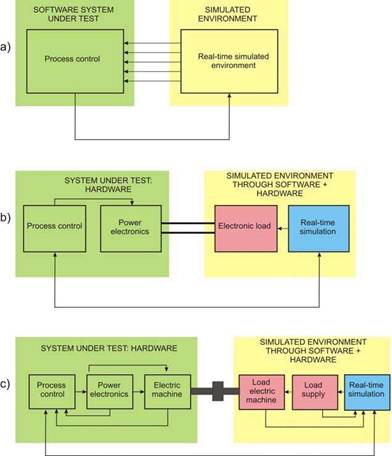
Fig. 1. Hardware-in-the-loop classification in a) signal, b) power and c) mechanical levels
3. Pure hardware: In the pure hardware case, the complete hardware setup of hybrid systems presents some drawbacks which cannot be ignored, such as high costs of the elements under test, the infrastructure and security requirements (especially for a hydrogen storage and supply system) and the complexity associated to the performance of the test when a high number of elements are involved. Moreover, each change in the simulation may require a re-design and new setup, with the associated time and cost.
Seen this classification, each HIL type can be applied depending on the final objective of the simulation. The power and mechanical level are particularly useful to simulate energy systems, such as those which can be found in an electric vehicle (batteries, ultracapacitors, fuel cells, etc.). Even if the mechanical HIL simulation can be more easily found in literature (Winkler & Gühmann, 2006) (Timmermans et al., 2007) it presents some drawbacks which can be solved in the HIL power level. These drawbacks are due to the presence of two electric machines, which increases the cost, infrastructure and complexity of the setup. Because the power level avoids the use of electric machines, the approach to the test bench developed can be focused on the energy systems tested, more than on the mechanical part.
Sizing the HIL simulation platform
To cope with systems where different currents, powers and voltage levels are involved, power engineers make an extensive use of the per-unit system (p.u.). The application of the p.u. system implies the adoption of a set of base values, to which the different magnitudes are referred. Therefore, the p.u. system variables become dimensionless values, allowing a much easier comparison between different alternatives and yielding more meaningful conclusions. The electric variables in a power system are power, voltage, current and impedance and a mathematical relationship between them can be found. As there are four different, but interdependent variables, it is a two degree of freedom system in which once two of the base values are defined, the other two can be obtained with:
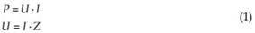
The choice of the base values is an arbitrary decision; however, for a particular component it is usual to select its rated values as base values. For example, in a generator with rated 200 MVA and 20 kV voltage, the base power and voltage can coincide with its rated values. Hence, the base current and impedance can be calculated as:
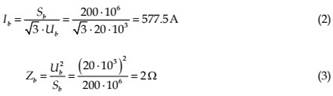
For this example, if an element consumes 20 MW, the p.u. power will be 0.1 p.u, which gives an understandable measure of the power consumed compared with the rated value.
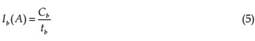
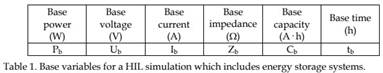
However, the classical version of the p.u. system does not include the presence of elements with energy storage, as therefore, a base capacity in A· h or C should be taken into account (Gauchia & Sanz, 2008). Hence, it is essential to introduce in the base system the concept of capacity and time, which are related with the discharge duration according to the Peukert equation (Peukert, 1897). C is the battery capacity, I the current and pc the peukert coefficient (usually between 0.5 and 2), which is unique for each technology and model. The equation reveals that the available capacity at constant discharge current is reduced for increasing discharge rates.

Therefore, a new set of base magnitude which includes a base capacity Cb related to a discharge time tb must be created. Known the base capacity and the discharge time (information which can be easily found in the data sheet handed by the manufacturer), the base current can be obtained with (5).
Therefore, the base system for the HIL simulation would include the variables in Table 1.
Any system attributes, as dynamic models, control, setup, results and conclusions expressed in p.u. values are also valid for absolute values, as it does not modify the nonlinear or particular characteristics of the element modelled. In the frame of a HIL simulation, the expression of variables in p.u. can be a very simple and effective way to introduce scaling factors to convert simulated physical variables into full-size physical ones.
Software and hardware elements of a HIL simulation
A HIL simulation is a flexible way of testing elements which are part of a complex system. Depending on the research interests, a decision must be made about which elements should be simulated and which should be included directly as hardware. When the focus is put directly on the energy systems, it is interesting to include one or more of them as hardware in order to have real information about its operation, whilst the rest of the system can be simulated through software and or hardware elements. When the energy system is the result of an integration of different energy elements, the possibilities of simulated/hardware elements increases significantly.
Case studied
The case studied is depicted in Fig. 2 and represents a hybrid electric vehicle, whose power source is the parallel combination of a fuel cell and battery. The hybrid combination of these two electrochemical energy systems allows to increase the vehicle range and to increase the efficiency, due to the variable driving cycles which can be found. Usually, a vehicle power load profile is formed by a relatively low base power (cruising) with very high abrupt power peak loads (acceleration and overtaking). In vehicles with internal combustion engines, the average power generated by the engine is considerably lower than its maximum power. If the internal combustion engine is substituted by a hybrid system fuel cell/energy storage, the primary system (fuel cell) can have a lower installed power due to the presence of the energy storage.
The fuel cell can supply the power needed for the base power load, however it cannot follow highly dynamic changes in the instantaneous power load. Fast energy storage devices, such as batteries or ultracapacitors can supply the power requested by the peak loads, but they suffer from serious capacity shortage for the supply of the long term energy (Nelson, 2000). As neither the fuel cell nor the fast energy storage devices can supply
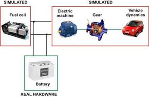
Fig. 2. Case studied:fuel cell-battery hybrid electric vehicle individually the whole power load, hybridization between both devices is needed. This is, of course, one of the possible alternatives, but it represents the most essential aspects of the problem.
The batteries present a wide variety of commercial technologies; however, especially designed for traction purposes lead-acid batteries are due to their maturity and robustness, as well as to their ability to supply very high current peaks. However, they may be replaced by ultracapacitors or by other battery technologies (Lukic et al., 2008), such as Ni-Mh or Liion, the latter being likely the most frequent choice in the next future. Once the elements of the hybrid system have been identified two relevant decisions must be made when designing a HIL simulation. The first one is related to which components should be simulated or implemented by hardware.
This choice is based on the flexibility, cost and complexity which each system adds to the whole HIL simulation. For example, a fuel cell is a complex and high cost system which needs special environments and installations due to the presence of hydrogen. Therefore, this system is a good candidate for being included as simulated in the HIL system. On the other hand, energy storage systems, such as batteries (or supercapacitors) are modular systems which do not require a specific installation and present a lower cost, simple operation and flexibility. Therefore, they are suitable for being part of the hardware systems in the HIL simulation, especially for electrical or electronic research laboratories, which are not specifically designed to operate with hydrogen-fed systems.
Vehicle modelling
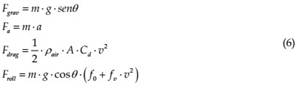
As seen in previous sections, the case studied is a fuel cell/battery vehicle, which is simulated through HIL, with a real battery and simulated fuel cell and vehicle. The simulated fuel cell and vehicle must be done in order to allow a feasible, robust and realistic approach to the real hybrid system. For the purpose of this type of simulation a simplified model for the mechanical part of the vehicle (vehicle forces, gear box and electric machine) may be used. The vehicle power requirements can be calculated through the resistance forces (Gillespie, 1992) which must be overcome by the vehicle power sources to move the vehicle at the desired speed. These resistance forces are normally calculated while the vehicle is being driven uphill, as shown in Fig. 3.
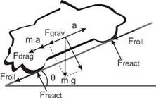
Fig. 3. Resistances to movement present in a vehicle driving uphill.
The resistance forces (6) represent the gravitational force, which depends on the vehicle mass m, the gravitational acceleration g and the slope angle Θ. Fa represents the acceleration resistance, which depends on the mass m and the vehicle acceleration a. The drag resistance Fdrag depends on the air density air, the vehicle frontal surface A, the drag coefficient Cd and the vehicle speed v. Finally, the rolling resistance Froll depends on the weight, the slope angle Θ, the static friction coefficient f0 and the dynamic friction coefficient fv (see Table 2).
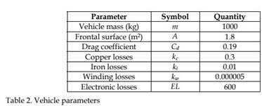
Electric power trains admit different electric machine technologies, such as induction machine, permanent magnets, switched reluctance, etc. as described by (Ehsani et al., 2007). When the focus is put on the implementation of a flexible test bench which allows both stationary and vehicular applications, the electric machine can be taken into account as a system which introduces an efficiency factor between the power requested by the vehicle and the power supplied by the fuel cell/battery system, centring the attention on the energy sources dynamic behavior and time window. In (7), T is the torque needed to move the vehicle at the requested speed; ω is the electric machine rotational speed, which depends on the gear ratio, kc, ki and kw represent the copper, iron and windage coefficient losses. The values for these coefficients are detailed in Table 2.
Vehicle simulator
The vehicle simulator presented by other authors, such as (Winkler & Gühmann, 2006) or (Timmermans et al., 2007) are constituted by electric machines working against a brake. The inclusion of this electric machine results in a high cost and complex HIL system.
The electric machine and brake can be substituted it by a controlled combination of programmable electronic load and power source. The dc electronic load (Chroma 63201) acts as a sink for the power generated by the energy sources, whilst the dc power source (Sorensen SGI) can generate regenerative braking by injecting power to the dc bus to which the energy sources are connected. It is important to take the regenerative braking into account as it has an important impact on the battery state of charge (SoC) and the vehicle range due to the recharging cycles. This vehicle simulator adds flexibility to the whole test bench, as any load power cycle (stationary or vehicular) can be simulated without altering the load simulator.
The layout of the vehicle emulator, shown in Fig. 4, is composed by a software and hardware simulation of the vehicle. The software part includes the driving cycle, vehicle resistive and traction forces, gear ratio and electric machine efficiency and torque. Once the speed driving cycle is transformed to a power or current profile, this profile is used to control externally both the electronic load and power source. The control of both the electronic load and power source is done analogically; through a 0-10 V signal which programs the equipment from 0-100% of its rated value.
The power generated by the simulated fuel cell and the physical battery is absorbed by the electronic load according to the programmed power cycle. The dc power source of the load
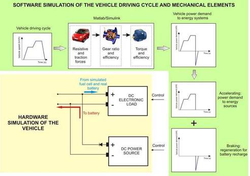
Fig. 4. Vehicle simulator proposed
simulator will only inject power in the dc bus during regenerative braking peaks. This power is used to recharge the battery. The power source is protected with a power diode which prevents current from sinking to the power source. The communication between the software and hardware part of the load simulator is done in real-time, as explained later.
Fuel cell modelling
This section presents a critical review of the fuel cell modelling techniques proposed by other authors, useful for the testing of hybrid energy systems.
The operational principle of fuel cells is based on electrochemical phenomena, but other processes, such as thermal, chemical, electric, fluid dynamic, etc. are also present. If all these phenomena should be taken into account at a time, the modelling process would result too complex and time consuming. When applying modelling and engineering processes, different approaches can be considered, depending on the final use given to the model developed. For example, fluid dynamic, thermal, chemical and electrochemical approaches are very adequate for the development stage of electrochemical system. But for the application stage, in which the electrochemical system has to interact with the load to which it is connected, an electric modelling of the system could be more adequate. Therefore, in this section we will focus on those models more suitable for a seamless integration into an electric simulation tool.
Engineering models would be useless if the numerical values of their parameters could not be determined through measures. For conventional systems (electric machines, combustion engines, transformers, etc.) whose mathematical models are perfectly defined, there are set of established tests, which allow obtaining the characteristics which define the system under study. Electrochemical systems can be also subjected to a series of tests which allow modelling their electrical behavior. Unlike conventional systems, the structure and mathematical models are still not universally defined, nor the test procedure or parameter obtention univocally established.
Modelling techniques: time vs. frequency domain test
The tests needed to obtain the dynamic models can be carried out either in the time or frequency domain. One of the most extended time domain tests is the current interruption test, whilst the most popular frequency domain test is the electrochemical impedance spectroscopy (EIS). The current interruption test is a time domain test in which the system under study is kept at its operation point (constant current load) until it reaches stationary state. Once reached, the current load is abruptly interrupted, allowing the study of the voltage evolution. Because electrochemical systems operate in direct current (dc), this test is carried out applying a dc current and measuring the dc voltage. The advantage of this modeling technique is its simplicity, both in setup and control. However, there are several drawbacks. One of them is that the model precision depends heavily on the correct identification of the point in which the voltage evolution changes from vertical to nonlinear. An imprecise calculation will cause the incorrect calculation of the voltage drops and the time constant. Finally, this method does not add significant information about the internal processes present in any electrochemical system. Some examples of the application of this method to fuel cells can be found in (Reggiani et al., 2007), and (Adzakpa et al., 2008). Whilst current interruption is carried out in the time domain and with direct current, EIS is a frequency domain test which needs the application of alternating current and voltage. EIS tests also seek to calculate the impedance of the system under study. But the most important advantages of frequency domain tests is the richer information obtained and the simpler data processing (if the adequate software is used).
Electrochemical systems present a nonlinear characteristic curve, but can be linearized if small variations are taken into account, as done with small signal analysis. To keep linearity during the tests, the ac signals applied are small enough (e.g. 5% of the rated voltage).
During EIS tests the ripple (either current or voltage) is applied to the electrochemical system. This ripple will cause the system to react, generating an ac voltage (if the excitation signal is current) or ac current (if the excitation signal is voltage). The ripple can be applied with a fixed (not usual) or variable frequency, which in the variable case can be programmed as a sweep. If the imposed ripple is current, it is said to be a galvanostatic mode EIS, whilst if it is a voltage signal it is called a potentiostatic mode. The selection criteria to chose between one mode or another is frequently the control mode of the system under test. For example, the fuel cell current is more easily controlled than the voltage. Hence, it would be easier to apply a galvanostatic (current control) mode.
Electrochemical systems generate direct current, therefore, it is unavoidable to have both dc and ac signals while carrying out EIS tests. The dc level is used to keep the electrochemical system at its operation point, but it is not considered for the impedance calculation, in which only the ac signals are involved. This implies that the dc level must be rejected before the ac impedance is calculated. A diagram explaining the whole process is presented in Fig. 5.
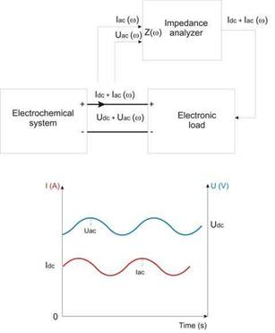
Fig. 5. EIS test procedure
EIS tests can be carried out with off-the-shelf equipment: electronic load, signal generator and voltage and current transducers. However, the subsequent impedance calculation and model extraction is time consuming and complex. Therefore, it is recommendable to use an impedance analyzer, which generates the excitation signal and calculates the complex impedance by measuring the current and voltage.
After the EIS test is carried out, the data must be processed. Normally the impedance analyzer includes a software package to do it. The data are rendered in a text file, which is traduced by the software to a Nyquist and Bode plot. Known these two plots, specially the Nyquist plot, the user can define an equivalent circuit, which the programme fits to the experimental results.
The most frequently used elements are resistances, capacitors and inductances. The resistance is represented by a point on the abscissa axis, with no imaginary part. Ideal capacitances or inductances correspond to vertical lines on the diagram. These ideal elements are rarely, if ever, found. It is more frequent to encounter real systems, which include the association of two or more of these elements, as presented in Fig. 6. The abscissa axis represents the real part of the complex impedance (Z’), whilst the ordinate axis is the imaginary part (Z”), so that the impedance is Z=Z’+jZ”. To facilitate the interpretation of the Nyquist plots, the upper part of the imaginary plot corresponds to the negative imaginary part (-Z”).
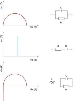
Fig. 6. Nyquist plots for combined ideal elements
For electrochemical systems, classic electric elements (resistances, capacitors and inductances) may not be enough to represent their internal behavior, due to, for example, diffusion phenomena. Most electrochemical systems use porous or rough materials for the electrode manufacture, which affect the diffusion of reactants. As stated by Barsoukov (Barsoukov & Macdonald, 2005), diffusion causes an effect similar to a finite transmission line: the answer of the output to an electric stimulation is delayed, compared to the input. Therefore, the electrochemical system will present a distributed equivalent circuit. The exact impedance cannot be represented as a infinite number of equivalent circuits, so for computational sake, it is normally limited to a finite number.
Fuel cell model
A PEM fuel cell is an electrochemical system which produces the electric power through its principal component: the stack. But the stack needs auxiliary systems, such as fan, compressor, filter, etc. in order to keep the stack environment in the correct operating conditions. Hence, the PEM fuel cell behavior presents thermal effects due to the heat generation, fluid dynamics present by the water and gas transport, electrochemical reactions in the stack, electrical phenomena, etc. The fluid, thermal and electrochemical approaches are specially useful for the development stage of fuel cells. But for the integration in its final application it is more useful an electric model, which can easily interact with the rest of electric models: electric machines, grid, power converters, etc. Therefore, in this chapter, an electric model will be developed. This electric model will adopt the form of an equivalent circuit which will be able to reproduce its voltage dynamic performance. The parameters of the resulting equivalent circuit will be obtained through electrochemical impedance spectroscopy EIS tests. Even if the work is applied to a PEM fuel cell due to its low operation temperature, which is ideal for transportation system, the experimental methodology and results can be extended to other technologies such as SOFC, DMFC, PAFC, etc.
The PEM fuel cell studied in this case is a 1.2 kW Nexa Ballard fuel cell which operates with direct gaseous hydrogen at its anode and air at its cathode.
The frequency electrochemical impedance spectroscopy (EIS) tests were carried out for 10, 20, 30, 40, and 50 A with a frequency interval of 0.5 Hz-6 kHz. The lower limit was chosen at 0.5 Hz as any frequency lower would increase the test time. The higher frequency limit was selected at 6 kHz as higher frequencies would not add relevant information to the model and as the fuel cell, by nature, will never supply high energy peaks during very fast transients. Fig. 7 represents the connections of the experimental test carried out. Throughout the tests the fuel cell is supplied with hydrogen stored at 200 bar. Moreover, the fuel cell communications systems needs a 24 V supply system, therefore a remote controlled power source is used.
The impedance analyzer controls the dc load through its software Zplot™, which establishes the ac and dc current which must be generated by the fuel cell. Both the current and voltage are measured by the impedance analyzer through the terminal V1 and V2 respectively. Later, the software ZView™ processes the experimental results.
The information obtained by ZView™ are the parameters of the equivalent circuit (depicted in Fig. 8) of the PEM fuel cell for the load current tested. Known all these parameters, the relationship of each parameter with the current can be obtained.
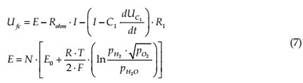
Where E represents the open circuit voltage of the fuel cell, which depends on the standard reversible voltage E0, the partial pressures of hydrogen pH2, oxygen pO2, and water pH20, as well as on the number of cells N, the ideal gas constant R, the temperature T, and the
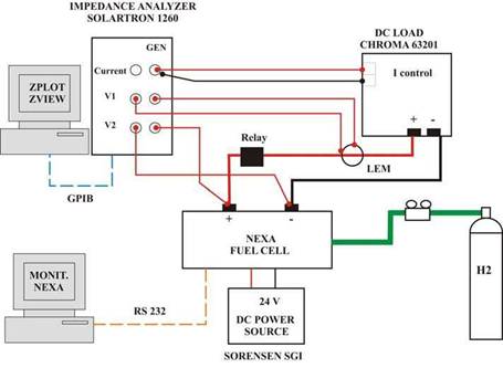
Fig. 7. EIS experimental test setup
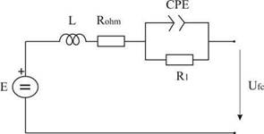
Fig. 8. Fuel cell equivalent circuit
Faraday constant F. The series resistance Rohm reflects the sum of the electrode internal resistance and the resistance to the flow of protons inside the membrane. L represents the inductive behavior of the fuel cell at high frequencies and the network R1CPE represent the dynamic behavior of the double layer capacitor which is situated between each electrode and the electrolyte. A constant phase element (CPE) is an element which represents the electrode roughness and inhomogeneous distribution of reactives on the electrode surface. As a CPE is not a physical electric element (Kötz & Carlen, 2000), it can be approximated by an equivalent capacitor C1. Once known the equivalent circuit of the fuel cell, the fuel cell output voltage can be calculated with:
A Matlab™/Simulink™ model of the fuel cell was programmed. In Fig. 9 experimental and model results are compared when a dynamic current is requested to the fuel cell. It can be observed that the model follows adequately the real fuel cell dynamic behavior. The discrepancy between the model and experimental results is due to the differences of the real and simulated temperature during very high currents. When the fuel cell stack reaches 65 ºC the cooling fan increases its duty cycle in order to cool the stack.
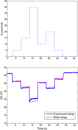
Fig. 9. Model validation
Fuel cell simulator
The fuel cell simulator is based on the dynamic nonlinear model obtained previously, which is fed to a dc power source which emulates its behavior. The fuel cell system simulator is formed by a programmable dc power source (Sorensen DCS20-150E) which is programmed with a 0-10 V signal for the output voltage and with a 0-10 V signal for the output current limit, allowing the voltage and current control of the fuel cell, just as it happens when the fuel cell is connected to a dc-dc power converter. These values are established by the control system, depending on the vehicle driving cycle and the battery state of charge, as explained later. The model presented in the previous subsection is implemented in Matlab™/Simulink™ and fed to the dc power source, as shown in Fig. 10. Just as in a physical fuel cell system, the power source which simulates the fuel cell operation is protected against sinking currents by a power diode. As in the case of the vehicle simulator, the interaction between the software and hardware simulation of the fuel cell system is done in real-time.
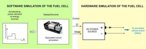
Fig. 10. Fuel cell simulator
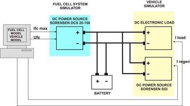
Fig. 11. HIL test bench power connections
HIL test bench
Power connections
The energy storage subsystem of this hybrid energy application consists of a Maxxima Exide-Tudor sealed lead-acid battery of 12 V, 50 Ah (20 h) connected in parallel to the dc bus. The power connections for the whole test bench are depicted in Fig. 11. As it can be observed, multiple power sources are connected in parallel. However, this presents no inconvenience in terms of voltage or current establishment. This is due to two facts. The first one is that the vehicle simulator (dc electronic load + power source) is current controlled, and therefore adapts to the voltage imposed by the hybrid energy system and hence, no ideal voltage sources are directly connected in parallel. The power source which simulates the fuel cell acts as a voltage or current source, depending on the load power requirements. Besides, both the simulated fuel cell and the battery show a non-negligible variable series impedances.
HIL acquisition system
An acquisition system is necessary to register the evolution of the different devices involved. LEM™ transducers are used to measure the dc bus voltage, as well as the simulated fuel cell, dc electronic load and dc power source which emulate the vehicle and battery current. The signals are acquired through an input/output board DS 2201, which is connected to its connector panel CP 2201. Both elements are part of a dSpace™ real-time control and acquisition system.
HIL control system
Hybrid systems accept a variety of control schemes, as for example (Thounthong et al., 2006), (Jiang et al., 2005), (Jiang & Fahini, 2009) or (Gao & Ehsani, 2009). The objective of the control system presented is to test the HIL test bench itself, in order to demonstrate its feasibility. Due to the fact that the energy system is hybrid between a simulated fuel cell and a physical battery, the control applied in this case will analyze and quantify the power share between the simulated fuel cell system and the real battery. Because the fuel cell system is not able to supply high energy peaks, the fuel cell system will be assigned the role of supplying the average power. With this strategy, the simulated fuel cell can be kept at or near the most efficient operation point. The power peaks will be supplied by the battery, which has a much faster response. The result is the simulated fuel cell feeding the average load power and recharging the battery during low current consumption periods, and the battery supplying power peaks and accepting energy during regenerative braking. Thence, it is possible to have a total control of the hybrid system by what could be called the “energy management mode” (EMM) of the system, which will depend on the type of control selected: fuel cell optimization, battery SoC, etc. The battery SoC at any instant must be calculated (8) and controlled.
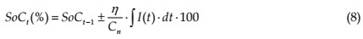
The SoC calculation takes into account the charging efficiency and the battery rated capacity Cn. As reflected in the second addend of (8), the charged capacity depends on the charge effciency. The sign of the second addend depends on the battery operation mode: it is positive for charge and negative for discharge.
The complete Matlab™/Simulink™ programme is shown in Fig. 12. The control system is implemented in a real-time platform as a general-purpose operating system does not have a consistent, repeatable, and known timing performance. The real-time platform is based on a dSpace™ Modular Hardware formed by an expansion box PX10, with a digital signal processor DSP DS 1006. The DSP communicates with the host computer through an optical cable and a PCI board. The dSpace and the host computer carry out task sharing, as the dSpace hardware performs the real-time calculation and the host computer provides the user interface and the experiment environment. The DSP DS 1006 is built around an AMD Opteron processor which runs at 3 GHz and has 256 MB as local memory for the execution of real-time models, 128 MB of global memory to exchange data with the host computer and 2 MB of flash memory. The I/O boards can be programmed using Matlab™/Simulink™ and Real Time Interface (RTI). The program developed is executed with a fixed step 1 ms and a fourth order Runge Kutta algorithm. The 1 ms time step selected is smaller than the vehicle (seconds), fuel cell (20 ms for the model used) and battery (10 ms for the battery used) time constant, and can therefore capture the dynamic operation of any system involved. Smaller time steps could lead to heavy experimental data files (e.g. over 1 million samples were recorded for each signal captured during the test carried out.) Fig. 13 presents the layout and photograph of the whole HIL simulation.
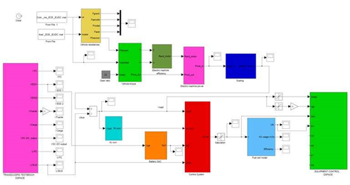
Fig. 12. HIL Matlab™/Simulink™ programme
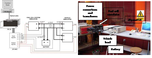
Fig. 13. Complete HIL setup and photograph
Energy management modes EMM’s
In a hybrid system, a wide range of control schemes could be implemented, depending on the objective: maximum range, minimum fuel consumption, minimum SoC variation, etc. This wide range of control schemes is due to the hybrid nature of the system, with one source able of supplying long term load (fuel cell) and another source capable of supplying shorter term loads (energy storage system). With these different time windows, control schemes may benefit one system but penalize the other. Therefore, some type of compromise should be reached.
In this work, two different and representative EMM’s of how a control scheme affects each system will be applied: the first one will reduce the hydrogen consumption and efficiently recharge the battery, whilst the second one will keep the battery SoC within an established interval. Of course, other control schemes could be tested.
For EMM1, the fuel cell output will vary between two different levels (one low level to reduce the fuel consumption and the maximum power point when the load current surpasses 100 A) while supplying the load and recharging the battery with a profile where the values are selected based on previous experiences with the battery. If the load current is smaller than the rated fuel cell current the battery starts a recharge cycle. The charge current depends on the battery SoC, as for increasing SoCs the battery voltage increases. The recommended charging voltage limit for this battery, as specified by the manufacturer, is 14.4 V. Due to the fact that the charge effciency decreases dramatically for high SoCs, the SoC is kept between 40 %-60 %, as in this interval there is no risk of overcharge or battery depletion, which would contribute to shorten the battery life due to gasification or sulphatation phenomena. The 60% upper limit for the SoC also assures that the battery will be always ready to accept power peaks during regenerative breaking.
For EMM2, the fuel cell will be kept at its maximum power point, both during the vehicle power following and during the battery recharge. Hence, the battery will have to deal with the peak transients. If during the driving cycle the battery voltage surpasses the manufacturer recommendation (max. 14.4 V or 1.2 p.u.) the control system will reduce the fuel cell reference (37.78 A or 2 p.u.) in order to reduce the charge regime or force the battery into a discharge cycle, which in both cases will lower the battery voltage.
In general, for both EMM’s, depending on the drive cycle, the battery could exceed the maximum 100% SoC if a low load or high regenerative breaking takes place. Hence, if the maximum SoC is exceeded the fuel cell reference will be reduced in order to force the battery into a discharge cycle. Also, the fuel cell will be in continuous operation, even during short stops, in order to recharge the battery. In this particular case, if the stop time exceeds 5 minutes the control system will stop the fuel cell. Moreover, if during the stop time the battery SoC exceeds the 80 %, the fuel cell will also stop.
HIL results
To test the p.u. HIL simulation presented, a driving cycle has been applied to the simulated system. The New European Driving Cycle (NEDC) simulates during 1225 seconds an urban and suburban route with frequent stops, as it can be seen in Fig. 14. The maximum speed is 120 km/h.
With this driving cycle the power requested to the downsized fuel cell/battery system is shown in Fig. 15. The maximum downsized power is 2500 W, which corresponds to a real 25 kW of the original application. As the simulation is carried out for a smaller system (10:1), the results presented are expressed in per-unit values.
The simulated fuel cell current is measured by a current transducer at the Sorensen DCS power source which emulates its behavior for both control schemes. The current profile is presented in per-unit values. For EMM1 in Fig. 16 the fuel cell current varies between 1.2 p.u. and 2 p.u., which are the two levels established. There is also a third level at 0.5 p.u., which corresponds to the battery recharge. For EMM2 in Fig. 17 the fuel cell is kept at a constant operation point (its maximum power transfer point), which corresponds with a 2 p.u. current, when the current is referred to the base system. These current values affect the hydrogen consumption, which is 2.5e-3 l/s for EMM1 and 3.7e-3 l/s for EMM2. Due to the fact that this constant operation of the fuel cell will affect the battery SoC and voltage, the control system will measure continuously the battery voltage. It can be observed in Fig. 16 that when the measured battery voltage surpasses 14.4 V (1.2 p.u.) the fuel cell current decreases in order to allow a battery discharge or reduce the recharge level. On the other hand, the bus voltage variation for control scheme 1 is lower, as it varies between 0.87 and 1.2 p.u.
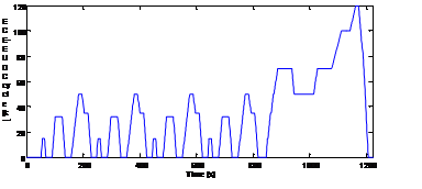
Fig. 14. Driving cycle
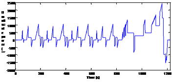
Fig. 15. Downsized power cycle (10:1)
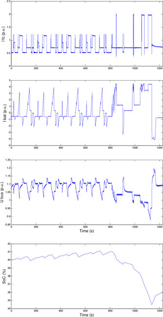
Fig. 16. Energy management mode 1
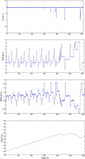
Fig. 17. Energy management mode 2
For both energy management modes the battery absorbs up to 5 p.u. The battery is recharged both from the fuel cell during low loads or during the regenerative braking. As the battery is reserved for the high peak currents, the bus voltage presents a variation around 1.07 p.u. for EMM1 and around 1.1 p.u. for EMM2. The voltage variation is of 0.33 p.u. for EMM1 and 0.37 p.u. for EMM2. This voltage variation is a normal situation for a battery, which needs to vary considerably its voltage in order to supply the current demanded during the charge/discharge cycles. This voltage variation is not so dramatic in other energy storage systems. For example, supercapacitors can supply or absorb hundreds of amperes during very short time intervals by just varying mV the supercapacitor voltage. The battery absorbs the frequent regenerative braking and fuel cell current which keeps the battery SoC. However, the two different energy managements affect the SoC in a considerable way. For EMM1 the SoC does not vary significantly during most part of the cycle, but collapses during the suburban section. EMM2 keeps the battery SoC within more appropriate values: 40% (0.4 p.u.) and 52% (0.52 p.u.), which avoids the battery depletion or overcharge. The fuel cell power varies around 2.2 p.u., which corresponds to 550 W in the downsized system and 5.5 kW in the real application. The battery power can reach nearly 5 p.u., which is 1250 W in the downsized system and 12.5 kW in the real system.
Conclusion
Hardware-in-the-loop simulation is a powerful tool for simulating systems with a high number of components, which may require a complex and expensive setup. In this chapter a HIL simulation has been applied to a fuel cell/battery hybrid vehicle. Unlike other authors, the vehicle simulation does not include an electric machine to reproduce the regenerative braking. A combined control of a dc electronic load and dc power source allows simulating both the vehicle power requirement and regenerative braking. This vehicle simulator can easily switch to a stationary load simulator by just changing the programmed power cycle. The hybrid fuel cell/battery system is setup as a combination of simulated and real hardware systems. The fuel cell simulator can be setup with a programmed dc power source which is able to reproduce the fuel cell voltage and current evolution. On the other hand, the battery is a simple and modular system which can be easily introduced as hardware.
The HIL simulation is carried out under a p.u. system, which allows to downsize the whole test bench and to study the hybridization between simulated fuel cell and battery. Moreover, different control strategies or EMM’s can be tested to simulate different scenarios.