Traffic data collection is an essential issue for road-traffic control departments, which need real-time information for traffic-parameter estimation: road-traffic intensity, lane occupancy, congestion level, estimation of journey times, etc., as well as for early incident detection. This information can be used to improve road safety as well as to make an optimal use of the existing infrastructure or to estimate new infrastructure needs. 

In an intelligent transportation system, traffic data may come from different kinds of sensors. The use of video cameras (many of which are already installed to survey road networks), coupled with computer vision techniques, offers an attractive alternative to other traffic sensors (Michalopoulos, 1991). For instance, they can provide powerful processing capabilities for vehicle tracking and classification, providing a non-invasive and easier to install alternative to traditional loop detectors (Fathy & Siyal, 1998; Ha et al., 2004).

Successful video-based systems for urban traffic monitoring must be adaptive to different traffic or environmental conditions (Zhu & Xu, 2000; Zhou et al., 2007). Key aspects to be considered are motion-based foreground/background segmentation ( Piccardi, 2004; Beymer et al., 2007; Kanhere & Birchfield, 2008), shadow removal algorithms ( Prati et al., 2003; Cucchiara et al., 2003), and mechanisms for providing relative robustness against progressive or sudden illumination changes. These video-based systems have to deal with specific difficulties in urban traffic environments, where dense traffic flow, stop-and-go motion profiles, vehicle queues at traffic lights or intersections, etc., would be expected to occur.

This chapter is focused on background subtraction, which is a very common technique for detecting moving objects from image sequences using a static camera. The idea consists of extracting moving objects as the foreground elements obtained from the “difference” image between each frame and the so-called background model of the scene ( Spagnolo et al., 2006). This model is used as a reference image to be compared with each recorded image. Consequently, the background model must be an accurate representation of the scene after removing all the non-stationary elements. It must be permanently updated to take into account the eventual changes in the lighting conditions or in the own background contents. Surveys and comparisons of different algorithms for background subtraction can be found in the literature (Piccardi, 2004; Chalidabhongse, 2003; Cheung & Kamath, 2004).

Regarding to the category of parametric background subtraction algorithms, in the simplest case, it is assumed that each background pixel can be modelled by a single unimodal

Source: Urban Transport and Hybrid Vehicles, Book edited by: Seref Soylu, 

 ISBN 978-953-307-100-8, pp. 192, September 2010, Sciyo, Croatia, downloaded from SCIYO.COM

probability density function. This is the case of the algorithm known as running Gaussian average (Wren et al., 1997; Koller et al., 1994), which is a recursive algorithm where a Gaussian density function is fitted for each pixel.

Temporal median filter is another common strategy which has been reported to perform better than those methods based on the average. The background estimate is defined for each pixel as the median of all the recent values (in the case of the non-recursive version of the algorithm). The assumption is that a background pixel must be clearly visible for more than 50% of the considered period (Cucchiara et al., 2003; Lo & Velastin, 2001; Zhou & Aggarwal, 2001).

Mixture of Gaussians (MoG) is another parametric strategy that has also been widely used (Stauffer & Grimson, 1999; Stauffer & Grimson, 2000; Harville, 2002). A single Gaussian density function for each pixel is not enough to cope with non-stationary background objects, such as waving trees or other natural elements. The idea under the MoG is to be able to model several background objects for each pixel. The achieved background tries to model the different intensities that can appear on each background pixel, using a mixture of n Gaussian density functions (Power & Schoonees, 2002). The optimal tuning of the parameter  set in this algorithm is considered not to be a trivial issue. In White & Shah (2007), an  automatic tuning strategy based on particle swarm optimization is proposed.

Another set of algorithms lay in the category of non-parametric algorithms. They are more suitable when it is assumed that the density function is more complex or cannot be modelled parametrically, since a non-parametric approach is able to handle arbitrary density functions. Kernel density estimation (KDE) is an example of non-parametric methods. It tries to solve a problem with the MoG and the other previous methods. These previous methods are able to effectively describe scenes with smooth behaviour and limited variation, as in the case of gradually evolving scenes. However, in the presence of a dynamic scene with fast variations or non-stationary properties, the background cannot be accurately modeled with a set of Gaussians. This technique overcomes the problem by estimating background probabilities at each pixel from many recent samples using kernel density estimation ( Elgammal et al., 1999). In Mittal & Paragios (2004), density functions are  estimated in a higher-dimensional space combining intensity information with optical flow, in order to build a method able to detect objects that differ from the background in either motion or intensity properties.

Another non-parametric approach is followed by the algorithm based in the called Codebook model ( Kim et al., 2005). In this case, the background model for each pixel is represented by a number of codewords (instead of parameters representing probabilistic functions) which are dynamically handled following a quantization/clustering technique. An important parallel issue in the conception of this technique is an appropriate colour modelling. Haritaoglu et al. (2000)  describe what they call W4 algorithm, where each background pixel is represented by a combination of the minimum and maximum values together with the maximum allowed change in two consecutive frames.

A different category of methods considers predictive strategies for modelling and predicting the state dynamics at each pixel. Some of them are based on Kalman filter (Karmann & Brandt, 1990; Koller et al., 1994), where intensity values and spatial derivatives are combined to form a single state space for background tracking. Alternatively, they may rely on the Wiener filter, as the  Wallflower algorithm (Toyama et al., 1999), or on more complicate models such as autoregressive models ( Monnet et al., 2003; Zhong & Sclaroff, 2003). Finally, we can also mention methods based on eigenspace representation, known as eigenbackgrounds ( Oliver et al., 2000), where new objects are detected by comparing the input image with an image reconstructed via the eigenspace.

Apart from background subtraction techniques, another extended approach is based on salient feature detection, clustering and tracking ( Beymer & Malik, 1996; Coifman et al., 1998). In this case, no background model has to be estimated and continuously updated. Instead, a bunch of prominent features that are expected to be stable along time are extracted from the vehicles’ image. Then, sophisticated spatiotemporal clustering algorithms are applied in order to group those features which are likely to belong to the same vehicle (proximity, motion coherence, velocity, can be used as clues). The main problem with these algorithms is that they assume that all the features for a given vehicle lie on the same plane, which can be acceptable for far viewpoints and small targets. Some other approaches try to overcome this problem projecting the extracted features onto a plane parallel to the road surface (Kanhere & Birchfield, 2008).

From an implementational point of view, video-based traffic equipments are frequently based on embedded processors with significant computational limitations. They have to perform several tasks in real time, including considerable amount of image processing ( Toral et al., 2009a). In this chapter, background subtraction algorithms with low computational requirements are considered for implementation on embedded processors. In particular, algorithms that allow reducing floating point computations to a minimum are preferable. This is the case of the above-mentioned median filter. However, the computation of the median value for each pixel from a number of recent samples is also a costly operation. A recursive algorithm, based on the sigma-delta filter, providing a very fast and simple approximation of the median filter with the additional benefit of having very low memory requirements, was proposed by McFarlane & Schofield (1995). In this algorithm, the running estimate of the median is incremented by 1 if the input pixel is above the estimate and decreased by one if over it. Manzanera and Richefeu (2004)  use a similar filter to compute the time-variance of the pixels, which is used for classifying pixels as “moving” or “stationary”. Recent enhancements of this algorithm have been proposed by Manzanera and Richefeu (2007) , with the addition of some interesting spatiotemporal processing, at the expense of a higher complexity.

In addition to the concern on computational efficiency, this chapter is specifically focused in urban traffic environments, where very challenging conditions for a background subtraction algorithm are common: dense traffic flow, eventual traffic congestions or vehicle queues are likely to appear. In this context, background subtraction algorithms must handle the moving objects that merged into the background due to a temporary stop and then become foreground again. Many background subtraction algorithms rely on a subsequent postprocessing or foreground validation step, using object localization and tracking, in order to refine the foreground detection mask. The aim of the proposed algorithm is to avoid the need of this subsequent step, preventing the background model to incorporate these objects which are stopped for a time gap and maintaining them as part of the foreground. At the same time, the algorithm should avoid the background model to get too obsolete after a change in the true background or in the illumination conditions. Consequently, special attention must be paid in deciding when and how updating the background model, avoiding “pollution” of the model from foreground slow moving or stopped vehicles, while preventing, at the same time, the background model to get outdated.

A new background subtraction algorithm based on the sigma-delta filter is described in this chapter and then compared with previous versions reported in the literature. A more reliable background model is achieved in common adverse conditions typical of urban traffic scenes, satisfying the goal of low computational requirements. Moreover, the implementation of the proposed algorithm on a prototype embedded system, based on an off-the-shelf multimedia processor, is discussed in this chapter. This prototype is used as a test-bench for comparison of the different background subtraction algorithms, in terms of segmentation quality performance and computational efficiency.

Sigma-Delta background estimation algorithms

Basic Sigma-Delta algorithm

The basic sigma-delta background estimation algorithm provides a recursive computation of a valid background model of the scene assuming that, at the pixel level, the background intensities are present most of the time. However, this model degrades quickly under slow or congested traffic conditions, due to the integration in the background model of pixel intensities belonging to the foreground vehicles. Table 1 describes the basic sigma-delta algorithm from Manzanera & Richefeu (2004) (a statistical justification of this method is given in Manzanera, 2007). For readability purposes, the syntax has been compacted in the sense that any operation involving an image should be interpreted as an operation for each individual pixel in that image.

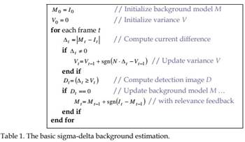
M_t represents the background-model image at frame t, I_t represents the current input image, and V_t represents the temporal variance estimator image (or variance image, for short), carrying information about the variability of the intensity values at each pixel. It is used as an adaptive threshold to be compared with the difference image. Pixels with higher intensity fluctuations will be less sensitive, whereas pixels with steadier intensities will signal detection upon lower differences. The only parameter to be adjusted is N, with typical values between 1 and 4. Another implicit parameter in the algorithm is the updating period of the statistics, which depends on the frame rate and the number of grey levels. This updating period can be modified by performing the loop processing every P frames, instead of every frame. The same algorithm computes the detection image or detection mask, D_t. This binary image highlights pixels belonging to the detected foreground objects (1-valued pixels) in contrast to the stationary background pixels (0-valued pixels). The described algorithm is, in fact, a slight variation of the basic sigma-delta algorithm, where the background model is only updated for those pixels where no detection is signalled, instead of doing it for all pixels. This selective updating is called relevance feedback and it is usually preferable, as it provides more stability to the background model.

Sigma-Delta algorithm with spatiotemporal processing

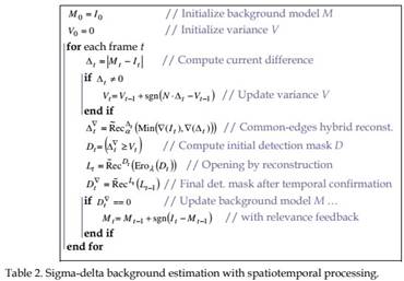
The basic sigma-delta algorithm only performs a strict temporal processing at the pixel level. Recent improvements suggest enhancing the method by adding some spatiotemporal processing (Manzanera & Richefeu, 2007) . The aim of the additional spatiotemporal processing is to remove non-significant pixels from the detection mask and to reduce the “ghost” and aperture effects. The “ghost effect” is the false detection produced by an object which suddenly starts moving after a motionless stay (a slow moving vehicle causes an effect similar to a ghost-like trail which can be apparent in the background model). The aperture effect produces poor detection for those objects with weak projected motion (for instance, objects moving nearly perpendicular to the image plane). The additional processing tries to improve and regularize the achieved detection through the following three operations: common-edges hybrid reconstruction, opening by reconstruction and temporal confirmation. These operations consider several common morphological operators ( Vincent, 1993; Heijmans, 1999; Salembier & Ruiz, 2002):

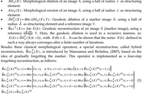
In these expressions, c and r refer to the column and row of each pixel in the image, respectively, while 1/α is the reconstruction radius replacing the structuring element. The three operations involved in spatiotemporal processing that make use of the detailed morphological operators are then:

1.        Common-edges hybrid reconstruction:  This step tries to make a reconstruction within Δ_t of the common edges in the current image and the difference image. It is intended to reduce the eventual ghost effects appearing in the difference image. ∇( )I must be understood as the gradient module image of I. The minimum operator, Min(), acts like an intersection operator, but working on gray-level values, instead of binary values. This operation retains the referred common edges belonging both to Δ_t and I_t. Finally, the _Rec^~ _α^Δt () operator performs the aforementioned reconstruction, trying to recover the whole object from its edges, but restricted to the

2.        Opening by reconstruction:difference image (Manzanera & Richefeu,  L_t = RecDt (Ero2007) λ(Dt. )). After obtaining the detection mask, this step is applied in order to remove the small connected components present in it. A binary erosion with radiusλ, Ero_λ( ) , followed by the usual geodesic reconstruction,

3.        Temporal confirmation:restricted to Dt, is applied.  D_t^∇ = RecLt (Lt−1 ) . The final detection mask is obtained after another reconstruction operation along time. This step, combined with the previous one, can be interpreted as: “keep the objects bigger than ┣ that appear at least on two consecutive frames”.

Table 2 describes the complete sigma-delta with spatiotemporal processing algorithm. Despite this rather sophisticated procedure, this algorithm also exhibits eventual problems due to its intrinsic updating period. For instance, it shows a limited adaptation capability to certain complex scenes in urban environments or, in general, scenes permanently crossed by lots of objects of very different sizes and speeds. In Manzanera and Richefeu (2007) , the authors suggest overcoming this problem using the multiple-frequency sigma-delta background estimation.

Multiple-frequency Sigma-Delta algorithm

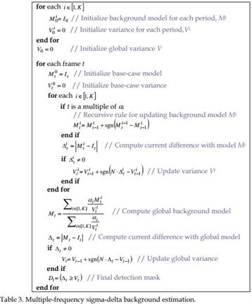
The principle of this technique is to compute a set of K backgrounds M_tⁱ, i∈[1,K] , each one characterized by its own updating period α_i. The compound background model is obtained from a weighted combination of the models in that set. Each weighting factor is directly proportional to the corresponding adaptation period and inversely proportional to the corresponding variance. The background model is improved, but at the expense of an increment in the computational cost with respect to the basic sigma-delta algorithm. Table 3 details an example of multi-frequency background estimation using K different periods

α₁<…<α_K.

In this case, the relevance feedback is not convenient due to fact of using several background models with different periods.

Sigma-Delta algorithm with confidence measurement

A different improvement of the basic sigma-delta background subtraction algorithm has been proposed by Toral et al., (2009b). The aim of this algorithm consists of trying to keep the high computational efficiency of the basic method, while making it particularly suitable for urban traffic environments, where very challenging conditions are common: dense traffic flow, eventual traffic congestions, or vehicle queues. In this context, background subtraction algorithms must handle the moving objects that merged into the background due to a temporary stop and then become foreground again. Many implementations overcome this problem with a subsequent post-processing or foreground validation step. The aim of this algorithm is to alleviate this subsequent step, preventing the background model to incorporate objects which are slow moving or stopped for a time gap. For this purpose, a numerical confidence level which is tied to each pixel in the current background model is introduced. This level quantifies the trust the current value of that pixel deserves. This enables a mechanism that tries to provide a better balance between adaptation to illumination or background changes in the scene and prevention against undesirable background-model contamination from slow moving vehicles or vehicles that are motionless for a time gap, without compromising the real-time implementation. The algorithm is detailed in Table 4. Three new images are required with respect to the basic sigma-delta algorithm: the frame counter image ( I_t^FC ), the detection counter image ( I_t^DC ) and the confidence image ( I_t^CON ).

 The variance image is intended to represent the variability of pixel intensities when no objects are over that pixel. In other words, the variance image will solely be determined by the background intensities, as a proper threshold should be chosen from that. A low variance should be interpreted as having a “stable background model” that has to be maintained. A high variance should be interpreted as “the algorithm has to look for a stable background model”. One of the problems of the previous versions of sigma-delta algorithms in urban traffic environments is that, as the variance grows when vehicles are passing by, the detection degrades because the threshold becomes too high. Then, it is necessary to perform a more selective background and variance update.

The main background and variance selective updating mechanism is linked to the so-called “refresh period”. Each time this period expires (let us say, each P frames), the updating action is taken, provided that the traffic conditions are presumably suitable. The detection ratio can be used as an estimation of the traffic flow. Notice that this is an acceptable premise if we assume that the variance threshold filters out background intensity fluctuations, as intended. Values of this detection ratio above 80% are typically related to the presence of stopped vehicles or traffic congestion over the corresponding pixels. If this is not the case, then the updating action is permitted.

On the other hand, high variance values mean that the capability for a proper evaluation of the traffic flow is poor, as the gathered information related to the detection ratio is not reliable. In this case, it is wiser not to recommend the updating action.

A parallel mechanism is set up in order to update the confidence measurement. This second mechanism is controlled by the so-called “confidence period”. This is not a constant period of time, but it depends on the confidence itself, for each particular pixel. The principle is that the higher the confidence level is, the lower the updating need for the corresponding pixel is. Specifically, the confidence period length is given by a number of frames equal to the confidence value at the corresponding pixel. Each time the confidence period expires, the

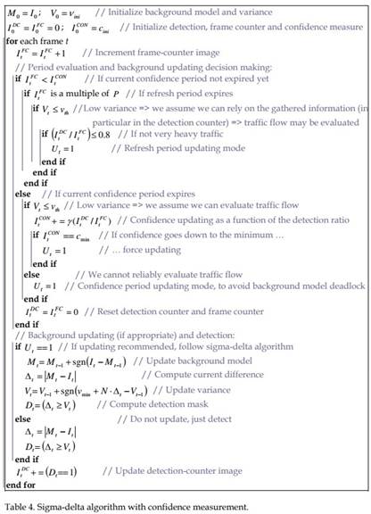
Table 4. Sigma-delta algorithm with confidence measurement. confidence measure is incrementally updated, according to an exponentially decreasing function of the detection ratio, d:

The gain α is tuned as the confidence maximum increment (when the detection ratio tends to zero), while β, defining the increment decay rate, has to be chosen such that negative increments are restricted to large detection rates.

The recommended values are, α = 11, so the maximum confidence increment is 10 frames, and β = 4 which adjusts the crossing of the function with -0.5 around 75%-80% of detection rates.

In case the confidence is decremented down to a minimum, background updating is forced. This is a necessary working rule since, in the case of cluttered scenes, for instance, the background model may not be updated by means of the refresh period. Thus, in that case, this underlying updating mechanism tries to prevent the model to get indefinitely locked in a wrong or obsolete background.

As a last resort, there is another context in which the updating action is commanded. This is the case when the confidence period expires but the detection capability is estimated to be poor. In such a case, as no reliable information is available, it is preferred to perform the background update. In fact, by doing otherwise, we will never change the situation, as the variance won’t be updated, hence the algorithm would end in a deadlock.

The confidence measurement is related to the maximum updating period. In very adverse traffic conditions, this period is related to the time the background model is able to keep untainted from the foreground objects. Let us suppose a pixel with correct background intensity and maximum confidence value, for instance, c_max = 125 frames. Then, 125 frames have to roll by for the confidence period to expire. If the traffic conditions do not get better, the confidence measure decreases until 124 and no updating action is taken. Now, 124 frames have to roll by for the new confidence period to expire. At the end, 125+124+123+…+10 = 7830 frames are needed for the algorithm to force the updating action (assuming minimum confidence value, c_min = 10). At the typical video rate of 25 frames per second, this corresponds to more than 5 minutes before the background starts becoming corrupted if the true background is seldom visible due to a high-traffic density. The downside is that, if we have a maximum confidence for a pixel with wrong intensity (for instance, if the background of the scene itself has experienced an abrupt change), also this same period is required for the pixel to be adapted to the new background. Nevertheless, if the change in the background is a significant illumination change, this problem can be alleviated in a further step by employing techniques related to shadow removal, which is beyond the scope of this paper (Prati et al., 2003; Cucchiara et al., 2003).

When the evaluation of the confidence measurement and the detection ratio recommend taking the updating action, the basic sigma-delta algorithm is applied. If no updating is required, the computation of the detection mask is just performed.

Comparative results

Qualitative performance analysis

A typical traffic urban sequence is used in this qualitative comparative study. In such scenes the background model from the basic sigma-delta algorithm quickly degrades, assimilating the slow moving or stopped vehicles. Another undesirable effect is that, in the long term, the corresponding variance values tend to increase immoderately in the areas with a higher traffic density. As the variance is used as a detection threshold, this detection is not very sensitive, producing a poor detection mask. This is illustrated in Fig. 1 for the traffic-light sequence. The first column of the figure shows the current image at frame 400 (that is 16 seconds after the sequence starts), which is the same for every row. The second column represents the current background model for each compared method. The third column represents the visual appearance of the variance image, and the fourth column represents the detection mask. The results shown in the first row corresponds to the basic sigma-delta algorithm, SD (parameter settings: N=4).  The second row corresponds to the sigma-delta with spatiotemporal processing, SDSP (parameter settings: N=4,α=1/8, λ=1 ), while the third row represents the results from the multiple-frequency sigma-delta background estimation, SDM (N=4, K=3 backgrounds models used, with adaptation periods: α₁ =1 , α₂ = 8 and α₃ =16 ). Finally, the fourth row corresponds to the sigma-delta with confidence , 

It can be seen that the adaptation speed of multi-frequency sigma-delta and the proposed method (when it is seeking for a new background) are similar. In particular, the moving vehicles present in the image at the beginning of the sequence have not been completely “forgotten” yet, producing the ghost vehicles noticeable in the case of these two algorithms. On the other hand, we can appreciate the effect of ghostly trails apparent in the background model, produced by the slow moving vehicles (or vehicles moving in a direction nearly perpendicular to the image plane), in the case of the two first algorithms.

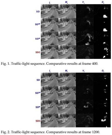
Fig. 2 illustrates another sample of the behaviour of these four algorithms at frame 1200 (48 seconds after the sequence start). In this case, some vehicles have been stopped in front of a red light for a maximum of 20 seconds approximately. It can be seen that these vehicles have been blended into the background model for both, the basic sigma-delta and sigma-delta with spatiotemporal processing, while they have been partially blended into the background for the multi-frequency sigma-delta. The sigma-delta with confidence measurement algorithm keeps this background model unpolluted from those stopped vehicles, being able to attain its full detection as foreground items. It can also be observed that the variance values have not been significantly increased in the region of the stopped vehicles, keeping the detection threshold conveniently sensitive.

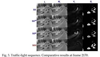
Next, the situation a few seconds later is shown in Fig. 3, corresponding to frame 2170, 86 seconds after the beginning of the sequence, and around 15 seconds after the vehicles in front of the traffic light started moving again. It can be seen that those vehicles have not been completely “forgotten” from the background model in the case of the basic sigmadelta, the sigma-delta with spatiotemporal processing and the multi-frequency sigma-delta algorithms. On the other hand, since this frame has been preceded by a significant traffic flow, the variance in the case of the first three algorithms has raised accordingly, producing a poor detection in the areas with higher variance. On the contrary, the sigma-delta with confidence measurement algorithm tries to keep the variance conveniently sensitive in those areas, as the variance is intended to represent the variability of the intensity levels of the background pixels only.

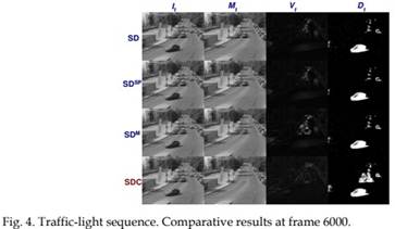
Finally, in Fig. 4, the situation 240 seconds after the sequence start is shown. This frame is part of the third red light cycle. The same comments made with respect to Fig. 2 are extensible to this later fragment of the sequence.

Quantitative performance analysis

There are different approaches to evaluate the performance of the background subtraction algorithms, from low-level, pixel-oriented evaluation to object-level or application-level evaluation. In the latter case, the goal-based evaluation of the foreground detection would be influenced by other higher level components of the application, e.g. a blob feature extraction module or a tracker module, which are out the scope of this paper. Consequently, in this section, a pixel-oriented evaluation has been preferred.

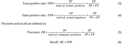
In a binary decision problem, the classifier labels samples as either positive or negative. In our context, samples are pixel values, “positive” means foreground object pixel, and “negative” means background pixel. In order to quantify the classification performance, with respect to some ground truth classification, the following basic measures can be used:

•       True positives (TP): correctly classified foreground pixels.

•       True negatives (TN): correctly classified background pixels.

•       False positives (FP): incorrectly classified foreground pixels.

•       False negatives (FN): incorrectly classified background pixels.

Using these basic measures, the true and false positive rates can be estimated:

Other measures for fitness quantification, in the context of background subtraction techniques, have been proposed in the literature (Rosin & Ioannidis, 2003; White & Shah, 2007; Ilyas et al., 2009). The following are some examples:

which combines precision and recall in the form of their harmonic mean, providing an index more representative than the pure PR and RE measures themselves.

The percentage of correct classification alone is very commonly used for assessing a classifier’s performance. However, it can give misleading estimates when there is a significant skew in the class distribution (Rosin & Ioannidis, 2003). In particular, if foreground elements are only present in a small part of the image, lets say 5%, there is not much difference in the achieved high ratings of this coefficient with respect to the case of simply classifying everything as background. Using additionally the Jaccard and Yule  coefficients (Sneath & Sokal, 1973) can reduce the problem, when there is a large volume of expected true negatives:

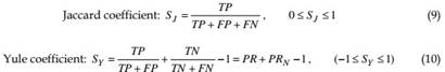
PR_N has to be understood as the precision in the background classification (negatives), in the same way PR is the precision in the foreground classification (positives). In its original form, the Yule coefficient is defined on the interval [-1,1]. The lower limit of this interval occurs when there are not matching pixels, while a perfect match would make the coefficient to hit the upper bound.

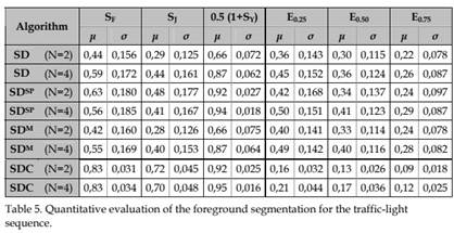
Finally, Ilyas et al. (2009) proposes a weighted Euclidean distance, considering the deviations of FPR and TPR from their respective ideal values, 0 and 1. It is defined as follows:

where γ (0< γ <1) is a weighting coefficient, that has to be adjusted according to the desired trade off between sensitivity and specificity. For instance, when a low false alarm rate is the priority, at the expense of loosing sensitivity, high values for this coefficient have to be chosen.

A representative ground truth dataset has been elaborated using the traffic light sequence. A number of samples from the traffic light sequence have been extracted and manually annotated using the publicly available annotation tool: InteractLabeler ( Brostow et al., 2009). One ground-truth frame for every 100 frames has been picked out, which corresponds to a 0.25 fps sampling rate. An initialization stage of around 20 seconds long is skipped over. 

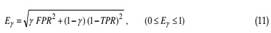
The following index sets have been considered as a valuable quantification of relative performance of each algorithm: S = {S_F , S_J , 0.5(1+ S_Y )}, E = {E_0.25, E_0.50, E_0.75)}. The first set includes fitness coefficients with ideal value equal to 1, while the second set includes fitness errors with ideal value equal to 0. The values of each one of these coefficients will be averaged for all the chosen frames. In addition, the typical deviation of each one is calculated. It can be noticed that the S_CC coefficient has been dropped from the analysis as, in agreement with the above comments, it exhibited a very poor sensitivity, yielding very high scores for every algorithm.

Table 5 details the average, ┤, and typical deviation, σ, for the chosen fitness indexes and the traffic light video sequence. According to the authors in Manzanera & Richefeu (2007), parameter N=2 was recommended for the SD, SDSP and SDM algorithms. However, in our experiments N=4 performed slightly better in some videos. Therefore, both values have been considered for each one of the four sigma-delta alternatives.

Results of the proposed sigma-delta algorithm with confidence measurement are clearly on top according to the fitness coefficients, both for N=2 and N=4. On the other hand, according to the fitness error coefficients, the proposed algorithm is significantly better than any of the other algorithms, featuring also a moderate typical deviation.

Hardware implementation

Embedded multimedia processors are expected to be on the basis of future ITS electronic equipments (Barrero et al., 2010). From a hardware point of view, a RISC processor is the core component of the multimedia processor. They can easily support an operating system for managing interfaces to communication channels like Ethernet and wireless devices, to massive storage devices like MMC/SD cards and USB pen drives, and to digital I/O or LCD screens. The multimedia processor also includes special support for video applications.

From a software point of view, embedded processors can incorporate not only computational intensive algorithms to allow traffic parameter estimation or incident detection, but also standard communication protocols, interface to data storage media (USB, MMC) and wireless connectivity (Bluetooth), FTP and SSH servers for software upgrading and a web server for remote configuration. Because of these complexities, it is advisable the use of an embedded operating system allowing the application programmers to focus on higher-level functionalities, like those based on artificial vision techniques. The selected operating system should support preemptive multitasking or multi-threading and device drivers for required connectivity. In this context, RISC processors are especially well suited for running such an operating system, offering a large spectrum of choices, both open source or proprietary.

A prototype based on the Freescale i.MX21 multimedia processor has been developed to deal with the computer vision functionality as well as the multimedia and networking capabilities (Fig. 5). The i.MX21 processor includes an ARM926EJ-S core, operating at 266 MHz. On-chip modules include LCD and memory card/secure digital controllers (MMC/SD), serial port controller (USB OTG), CMOS sensor interface, and enhanced MultiMedia Accelerator (eMMA), which consists of a video Pre-processor (PrP) unit, an Encoder (ENC) and a Decoder (DEC) module, and a Post-processor (PP) unit. MPEG-4 and H.263 protocols are supported as well as real-time encoding/decoding of images from 32×32 pixels up to CIF format at 30 frames per second. The PrP resizes input frames from memory or from the CMOS sensor interface, and performs color space conversion. The PP module takes raw images from memory and performs additional processing to de-block, dering, resize, and color space conversion on the decoded frames for MPEG-4 video streaming. The prototype board is also provided with mini USB and SD card connector, RJ45 Ethernet connector, Bluetooth expansion connector, and a coaxial connector, which provides the analog signal to a video decoder chip.

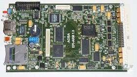
Fig. 5. Hardware prototype.

Although a multitude of embedded operating systems are currently available (Wind River’s VxWorks, Microsoft Windows CE, QNX Neutrino, etc), Linux is firmly in first place as the operating system of choice for smart gadgets and embedded systems (Toral et al., 2009c). All embedded operating systems require a considerable effort of customization, because they incorporate a wider variety of input/output devices than typical desktop computers. As a consequence, it is necessary to adapt the operating system to the particular features of the selected processor. Fortunately, Linux comes under a GPL license and the community of support around Linux ports are of great help during the customization task. Linux runs on multiple embedded architectures, but ARM and PowerPC are the best supported processors. Besides, Linux support multitasking/multithreading, allowing several processes and services running in concurrent operation. In the proposed application, the i.MX21 video processor is running under ARM Linux (kernel 2.4.20). The main process corresponds to the background model estimation, but several processes executing additional services are in concurrent operation:

•       A HTTP server for configuration and supervision purposes.

•       A Web command server module, in charge of processing specific requests from the configuration web page.

•       A SSH server for remote logging into the system.

•       A FTP server for upload and download operations.

•       A watchdog process for rebooting the system when a periodic signal is not received from the main process. 

•       A video delivery process for video compression and delivery using an Ethernet interface.

All the sigma-delta algorithms have been programmed using C++ programming language. Full resolution, gray-scale images 720×576 pixels are subsampled to resolution 360×288 before being processed. Table 6 shows the time requirements of each one of the considered algorithms, while performing on a typical traffic sequence.

Considering the average time or the effective velocity columns, the basic sigma-delta algorithm is the less time consuming, as expected, followed by the proposed algorithm. The multifrequency sigma-delta takes around 2.5 times more than the proposed algorithm, while the sigma-delta with spatio-temporal processing is about 13 times slower. On the other hand, regarding to the maximum cycle time, we can see that both, the multifrequency sigma-delta and the SDC algorithm, double their respective average times, while the sigmadelta with spatio-temporal processing triplicate its average time in the worst case. Furthermore, the basic sigma-delta algorithm and the enhanced version with confidence measurement have the benefit of a much lower typical deviation in its cycle time. 

Algorithm	Tmin (ms)	Tmax (ms)	Tmean (ms)	Tdesv (ms)	Speed (fps)
SD	(N=4)	< 1	31	11,37	6,84	87,95
SDSP	(N=4)	218	1201	387,07	52,48	2,54
SDM	(N=4)	31	172	77,64	14,04	12,88
SDC	(N=4)	15	62	30,18	5,71	33,14

Table 6. Time requirements of each algorithm.

Applications

The main process of the prototype corresponds to vision-based vehicle detection system. This detection relies on the so called detection areas. Each one of these areas or regions is a user-configurable polygon with an arbitrary shape or size, and an associated functionality. Three kinds of detection regions have been programmed: presence, directional and queue regions, allowing the estimation of useful traffic information. The functionality of these regions is clarified below:

•       Presence-detection regions. They may be considered as virtual loop detectors, quite similar to the traditional on-the-road loop detectors buried under the road surface (Michalopoulos, 1991). These non-invasive loop detectors generate a binary output (vehicle presence or absence) depending on a configurable threshold, and incorporate a software vehicle counting functionality.

•       Directional-detection regions. The directional regions are also used for counting vehicles. Unlike the previous type, its goal is to estimate the vehicle running direction, checking how close it is to the configured direction associated to the region. Depending on the agreement of both directions, the vehicle is counted or ignored. This kind of regions is useful for selective vehicle counting in or near intersections, one-way violation detections or restricted turn infringements.

•       Queue-detection regions. The queue regions are intended to estimate vehicle queue length and queuing frequency, typically, in front of a traffic light. A binary output can be also associated with these regions, indicating whether the instantaneous queue length is above or below a configured threshold.

This main process requires the complete configuration of the scene, which can be made via the HTTP server running in the multimedia processor. Fig. 6 illustrates one of the screens in the system’s configuration web page.

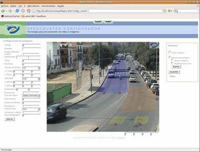
Fig. 6. Equipment configuration web site.

The image on the centre of the web page shows a snapshot of a video stream delivered by the real-time application. Several detection regions have been defined: two presencedetection regions in yellow configured to count vehicles running on both lanes, one directional detection region in pink configured to count vehicles coming from the right side of the intersection, and two queue regions in blue in front of a traffic light. Associated to each detection area, both instantaneous and time-aggregated data can be obtained:

•       Presence-detection regions: occupancy and vehicle counting data during the aggregation period. The occupancy gives an estimation of the percentage of time the presence level is above the configured threshold (presence on).

•       Directional-detection regions: directional vehicle counting data.

•       Queue-detection regions: queue counting data (number of times the queue has exceeded the configured threshold during the aggregation period), time ratio the queue is above the configured threshold (queue on) and average queue length.

Instantaneous data overlaid on the real-time image (upper left corner of the image of Fig. 6), and produce digital outputs emulating traditional detectors. The aggregated data can be also recorded on a log file (which is updated at the end of each aggregation period), and then downloaded using the FTP server.

Conclusion

In this chapter, several background modelling techniques have been described, analyzed and tested. In particular, different algorithms based on sigma-delta filter have been considered due to their suitability for embedded systems, where computational limitations affect a real-time implementation. A qualitative and a quantitative comparison have been performed among the different algorithms. Obtained results show that the sigma-delta algorithm with confidence measurement exhibits the best performance in terms of adaptation to particular specificities of urban traffic scenes and in terms of computational requirements. A prototype based on an ARM processor has been implemented to test the different versions of the sigma-delta algorithm and to illustrate several applications related to vehicle traffic monitoring and implementation details.