The major components of an electric vehicle system are the motor, controller, power supply, charger and drive train (wry, 2003). Fig. 1 demonstrates a system model for an electric vehicle. Controller is the heart of an electric vehicle, and it is the key for the realization of a high-performance electric vehicle with an optimal balance of maximum speed, acceleration performance, and traveling range per charge.
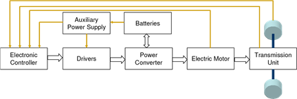
Fig. 1. Major components in an electric vehicle
Control of Electric Vehicle (EV) is not a simple task in that operation of an EV is essentially time-variant (e.g., the operation parameters of EV and the road condition are always varying). Therefore, the controller should be designed to make the system robust and adaptive, improving the system on both dynamic and steady state performances. Another factor making the control of EV unique is that EV’s are really “energy-management” machines (Cheng et al., 2006). Currently, the major limiting factor for wide-spread use of EV’s is the short running distance per battery charge. Hence, beside controling the performance of vehicle (e.g., smooth driving for comfortable riding), significant efforts have to be paid to the energy management of the batteries on the vehicle.
However, from the viewpoint of electric and control engineering, EV’s are advantagous over traditional vehicles with internal combustion engine. The remarkable merit of EV’s is the electric motor’s excellent performance in motion control, which can be summerized as (Sakai & Hori, 2000): (1) torque generation is very quick and accurate, hence electric motors can be controlled much more quickly and precisely; (2) output torque is easily comprehensible; (3) motor can be small enough to be attached to each wheel; (4) and the controller can be easily designed and implemented with comparatively low cost.
Source: Urban Transport and Hybrid Vehicles, Book edited by: Seref Soylu,
ISBN 978-953-307-100-8, pp. 192, September 2010, Sciyo, Croatia, downloaded from SCIYO.COM
Hence, in recent years, there is quite a lot of researches in the exploring advanced controll strategies in electric vehicles. As the development of the high computing capability microprocessor, such as DSP (Digital Signal Processor), it is possible to perform complex control on the electric vehicle to achieve optimal performance (Liu et al., 2004). These capabilities can be utilized to enhance the performance and safety of individual vehicles as well as to operate vehicles in formations for specific purposes (Lin & Kanellakopoulos, 1995). Due to the complex operation condition of electric vehicle, intelligent or fuzzy control is generally used to increase efficiency and deal with complex operation modes (Poorani et al., 2003; Khatun et al., 2003). However, it is essential to establish a model-based control for the EV system, and systematically study the characteristics to achieve optimal and robust control. This chapter will mainly focuses on model-based control design for EV’s and the implementation of the platform for realization of variant control strategies.
Modeling of electric vehicle
Generally, the modelling of an EV involves the balance among the forces acting on a running vehicle, as shown in Fig. 2. The forces are categorized into road load and tractive force. The road load consists of the gravitational force, hill-climbing force, rolling resistance of the tires and the aerodynamic drag force. Consider all these factors, a vehicle dynamic model that governs the kinetics of the wheels and vehicle can be written as (wry, 2003):
F = μrrmg + ![]() 1 ρAC vd 2 + mgsinφ+ m
1 ρAC vd 2 + mgsinφ+ m ![]() dv (1)
dv (1)
2 dt
Where, m is the mass of the electric vehicle; g is the gravity acceleration; v is the driving velocity of the vehicle; μrr is the rolling resistance coefficient; ρ is the air density; A is the frontal area of the vehicle; Cd is the drag coefficient; and φ is the hill climbing angle.
The rolling resistance is produced by the flattening of the tire at the contact surface of the roadway. The main factors affecting the rolling resistance coefficient μrr are the type of tyre and the tyre pressure. It is generally obtained by measurement in field test. The typical range is 0.005-0.015, depending on the type of tyre. The rolling resistance can be minimized by keeping the tires as much inflated as possible.
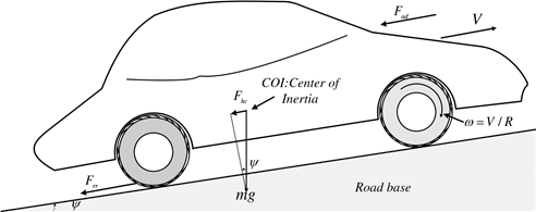
Fig. 2. External forces applied on a running vehicle
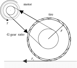
Fig. 3. A simplified model for motor driving tyre
In equation (1), the first term corresponds to the rolling resistance force; the second term corresponds to the aerodynamic drag force; the third term corresponds to the hill climbing force; and the forth term corresponds to the acceleration force.
This resultant force F, will produce a counteractive torque to the driving motor, i.e., the tractive force. For vibration study, the connection between the driving motor and the tyre should be modeled in detail. Interested readers are refered to (Profumo et al., 1996). In this chapter, a simplified model, as shown in Fig. 3, will be used. With this simplified model, the relationship between the tractive force and the torque produced by the motor can be obtained as:
TL = F ⋅ ![]() r (2)
r (2)
G
Where r is the tyre radius of the electric vehicle, G is the gearing ratio, and TL is the torque produced by the driving motor.
Electric motor and their models
Presently, brushed DC motor, brushless DC motor, AC induction motor, permanent magnet synchronous motor (PMSM) and switched reluctance motor (SRM) are the main types of motors used for electric vehicle driving (Chan, 1999). The selection of motor for a specific electric vehicle is dependent on many factors, such as the intention of the EV, ease of control, etc.
In control of electric vehicle, the control objective is the torque of the driving machine. The throttle position and the break is the input to the control system. The control system is required to be fast reponsive and low-ripple. EV requires that the driving electric machine has a wide range of speed regulation. In order to guarantee the speed-up time, the electric machine is required to have large torque output under low speed and high over-load capability. And in order to operate at high speed, the driving motor is required to have certain power output at high-speed operation. In this chapter, the former four types of motors that can be found in many applications will be discussed in detail.
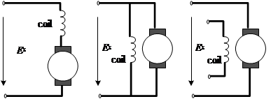
Fig. 4. Three types of winding configuration in DC motor
Brushed DC motor
Due to the simplicity of DC motor controlling and the fact that the power supply from the battery is DC power in nature, DC motor is popularly selected for the traction of electric vehicles. There are three classical types of brushed DC motor with field windings, series, shunt and ‘separately excited’ windings, as shown in Fig. 4. The shunt wound motor is particularly difficult to control, as reducing the supply voltage also results in a weakened magnetic field, thus reducing the back EMF, and tending to increase the speed. A reduction in supply voltage may, in some circumstances, have very little effect on the speed. The separately excited motor allows one to have independent control of both the magnetic flux and the supply voltage, which allows the required torque at any required angular speed to be set with great flexibility. A series wound DC motor is easy to use and with added benefit of providing comparatively larger startup torque. A (series) DC motor can generally be modeled as (Mehta & Chiasson, 1998):
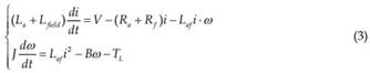
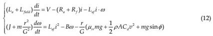
Where: i is the armature current (also field current); ω is the motor angular speed; La, Ra, Lfield, Rf are the armature inductance, armature resistance, field winding inductance and field winding resistance respectively; V is the input voltage, as the control input; Laf is the mutual inductance between the armature winding and the field winding, generally non-linear due to saturation; J is the inertia of the motor, including the gearing system and the tyres; B is the viscous coefficient; and TL is representing the external torque, which is quantitatively the same as the one aforementioned.
Brushless DC motor
The disadvantages of brushed DC motor are its frequent maintenance and low life-span for high intensity uses. Therefore, brushless DC (BLDC) motor is developed. Brushless DC motors use a rotating permanent magnet in the rotor, and stationary electrical magnets on the motor housing. A motor controller converts DC to AC. This design is simpler than that of brushed motors because it eliminates the complication of transferring power from outside the motor to the spinning rotor. Brushless motors are advantageous over brushed ones due to their long life span, little or no maintenance, high efficiency, and good performance of timing. The disadvantages are high initial cost, and more complicated motor speed controllers (Wu et al., 2005).
A BLDC motor is composed of the motor, controller and position sensor. In the BLDC motor, the electromagnets do not move; instead, the permanent magnets rotate and the armature remains static. The rotor magnetic steel is radially placed, and the permanent magnets (generally Neodymium-iron-boron: NdFeB) are installed on the surface. The magnetic permeability of such permanent magnets is close to that of air, hence can be regarded as part of the air gap. Hence, there is no salient pole effect, so that the magnetic field across the air gap is uniformly distributed. The position sensor functions like the commutator of brushed DC motor, reflecting the position of the rotor and determining the phase of current and space distribution of magnetic force.
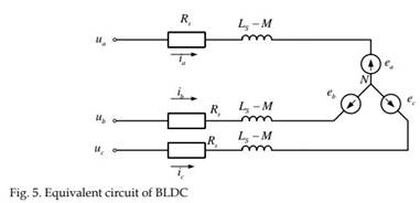
The BLDC motor is actually an AC motor. The wires from the windings are electrically connected to each other either in delta configuration or wye (“Y”-shaped) configuration. In Fig. 5, an equivalent circuit of wye-connected BLDC is shown. With this configuration, the simplified model can be obtained as:
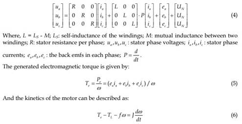
Where, ω: the angular velocity of the motor; Te, TL: electromagnetic torque of the motor and the load torque; Pe: electromagnetic power of the motor; J: moment of inertia; f: friction coefficient.
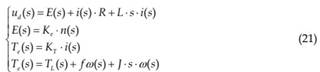
Under normal operation, only two phases are in conduction. Then the voltage balance equation, back EMF equation, torque equation, and kinetic equations that govern the operation of a WYE connected BLDC motor can be obtained as:
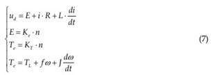
Where, ud: the voltage across the two windings under conduction; E: the back EMF of the two windings under conduction; KT: torque coefficient, and Ke: back EMF coefficient. It is shown that, in BLDC motors, current to torque and voltage to rpm are linear relationships.
Permanent magnet synchronous motor
A permanent magnet synchronous motor is a motor that uses permanent magnets to produce the air gap magnetic field rather than using electromagnets. Such motors have significant advantages, such as high efficiency, small volume, light weight, high reliability and maintenance-free, etc., attracting the interest of EV industry. The PMSM has a sinusoidal back emf and requires sinusoidal stator currents to produce constant torque while the BDCM has a trapezoidal back emf and requires rectangular stator currents to produce constant torque. The PMSM is very similar to the wound rotor synchronous machine except that the PMSM that is used for servo applications tends not to have any damper windings and excitation is provided by a permanent magnet instead of a field winding. Hence the d, q model of the PMSM can be derived from the well known model of the synchronous machine with the equations of the damper windings and field current dynamics removed.
In a PMSM, the magnets are mounted on the surface of the motor core. They have the same role as the field winding in a synchronous machine except their magnetic field is constant and there is no control on it. The stator carries a three-phase winding, which produces a near sinusoidal distribution of magneto motive force based on the value of the stator current. In modeling of rotating machines like PMSM, it is a general practice to perform Park transform and deal the quantities under dq framework. The dqo transform applied to a three-phase quantities has following form:
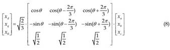
Where, the x can be voltage u or current i.
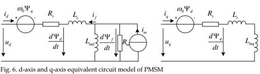
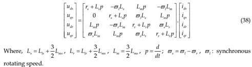
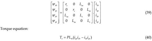
Under the dq0 framework, the equivalent circuit of d-axis and q-axis circuits of a PMSM motor is shown in Fig. 6, and the model of a PMSM can be written as (Cui et al., 2001):
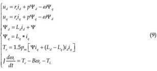
Where, Ψd, Ψq: the flux linkages of d-axis and q-axis respectively; Ld, Lq: self inductance of dq axes; id, iq: dq-axis current; ud, uq: dq-axis voltage; ωr: angular velocity of rotor; rs: stator resistance; pm: number of poles; Ψ: flux linkage produced by the rotor permanent magnet; Te: motor torque; TL: load torque; J: moment of inertia; B: friction coefficient; p: differential operator.
The first two equations are the equations for stator voltage, the next two equations are about the magnetic flux linkage, the fifth equation is about the calculation of torque, and the last equation is about the kinetics of the motor.
Induction motor
Induction machines are among the top candidates for driving electric vehicles and they are widely used in modern electric vehicles. Some research even concludes that the induction machine provides better overall performance compared to the other machines (Gosden et al., 1994).
An induction motor (or asynchronous motor or squirrel-cage motor) is a type of alternating current motor where power is supplied to the rotor by means of electromagnetic induction. It has the advantages such as low-cost, high-efficiency, high reliability, maintenance-free, easy for cooling and firm structure, etc. making it specially competitive in EV driving. In induction motor, stator windings are arranged around the rotor so that when energised with a polyphase supply they create a rotating magnetic field pattern which sweeps past the rotor. This changing magnetic field pattern induces current in the rotor conductors, which interact with the rotating magnetic field created by the stator and in effect causes a rotational motion on the rotor.
AC induction motor is a time-varying multi-variable nonlinear system, hence the modeling task is not easy. For simplicity, following assumptings have to be made:
• Magnetic circuit is linear, and saturation effect is neglected;
• Symmetrical two-pole and three phases windings (120° difference) with edge effect neglected;
• Slotting effects are neglected, and the flux density is radial in the air gap and distributed along the circumference sinusoidally;
• Iron losses are neglected.
With such assumptions, the physical model of an induction motor can be given as shown in Fig. 7. The three-phase stators are fixed on A, B and C axes, which are stationary reference frames. The three-phase rotor windings are fixed on a, b and c axes, which are rotating frames. Hence the equations governing the dynamics of the induction motor can be given as (Dilmi & Yurkovich, 2005):
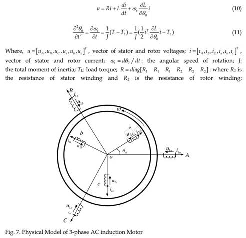
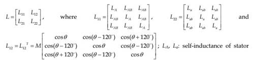 and rotor; LAB, Lab: mutual inductance of stators and rotors respectively; M: mutual inductance between stator and rotor.
The first equation is the voltage equation and the second equation is the kinetic equation of the motor.
Controller design of electric vehicle driven by different motors
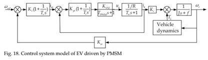
Fig. 8 shows a universal framework for electric vehicle controller. The vehicle is driven by a motor, which is supplied by the battery through a controlled power circuit. Other than circuit for control of the motor, there is quite a lot of auxiliary control for auto electronics. The control strategies are implemented in the microprocessor, such as DSP (Digital Signal Processor).
Control of electric vehicle is essentially the control of motor. In Fig. 8, only the motor and its associated driving power circuit will be replaced with different motors. With different motors, it is necessary to use different control strategies. However, it is not possible to include all type of motor and control strategies in one book. Hence, in this chapter, only one typical controller or control strategy will be presented. It is noticed that (Chan, 1999) generally PWM control is used for DC motor, while variable-voltage variable-frequency (VVVF), FOC (field-oriented control) and DTC (direct torque control) are used for induction motor. And some traditional control algorithms, such as PID, cannot satisfy the requirements of EV control. Many modern high-performance control technologies, such as adaptive control, fuzzy control, artificial neuro network and expert system are being used in EV controllers.
Driven by brushed DC motor
In this subsection, the controller design for an EV driven by series wound DC motor will be discussed. When the electric vehicle is driven by a series wound DC motor, the overall system model is the combination of (1) and (3):
In this case, a model-based controller can be designed. Unlike other applications in which the system generally operates around the equilibrium point, the operation of EV may take a very wide range (e.g., from zero to full speed). Hence, it is essentially to design EV controller with nonlinear control techniques. The model-based controller is very sensitive to the uncertainties in the parameters. Many parameters in the complex vehicle dynamics
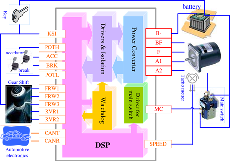
Fig. 8. Model of electric vehicle controller cannot be precisely modeled and some parameters may vary due to the varying operation conditions. For example, the resistance in the armature winding of a motor would change as the operation temperature varies. Hence, when designing the controller, the robustness of the controller should be first considered. In this subsection, a nonlinear robust and optimal controller (Huang et al., 2009) will be discussed.
For the convenience of designing nonlinear controller, first change the model in (12) into the following format:
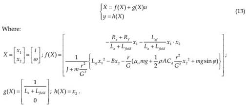
In order to consider the uncertainties of the system, further change the form of (13) into:
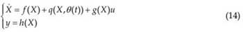
f(X), g(X) and h(X) are the same as in previous section. q(X,θ(t)) is used to include the model uncertainties, where θ(t) is the uncertainty vector. In the model described above, the rolling resistance coefficient and aerodynamic dragging coefficients cannot be precisely modeled. These coefficients are always varying along the moving of the vehicle (e.g., due to wind). Also, the resistance of the windings is also varying due to the variation of temperature. Hence, q(X,θ(t)) can be modeled as:
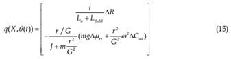
Where, ΔR, Δμrr and ΔCad are the uncertainties in winding resistance, rolling resistance coefficient and aerodynamic dragging coefficient respectively, with ΔRm, Δμrr _ m and ΔCad _ m representing their maximum uncertainties.
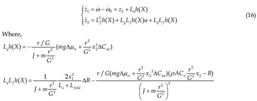
By using the similar coordinate transformation, we have,
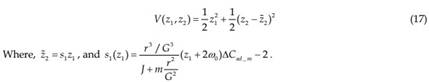
Hence, by using the recursive backstepping design method with robust control system (Marino & Tomei, 1993; Freeman & Kokotovic, 1996), one can select a robust control Lyapunov function (rclf) as:
Then, the control law in (18) can robustly stabilize the electric vehicle system with any parametric uncertainties:
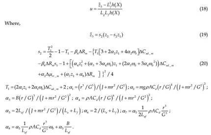
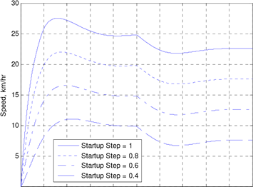
Fig. 9 shows the robustness test result of a controller designed for a light-weighted EV, compared against a regular PID controller, with parameters as specified in Table 1. To facilitate the graphical representation, the sudden change in hill climbing angle (0.1 rad) is
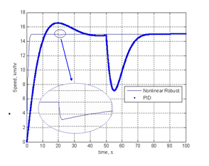
Fig. 9. Robustness test of the non-linear robust controller
applied on the nonlinear robust controller system at t=20 s and on the double-loop PID controller at t=50 s. Shown in Fig. 10 is the excellent robust performance of the designed controller under parameter uncertainties. The test is performed with the arbitrary combinations (i.e., uncertainty in single parameter, two parameters and three parameters) of ±10% uncertainty in the aforementioned three uncertain parameters. Again, for comparison purpose, the performance of (double loop) PID controller and the nonlinear optimal controller are plotted in Fig. 11 and Fig. 12 respectively.
To systematically test the performance, the New European Driving Cycle (NEDC) is used. The New European Driving Cycle is a driving cycle consisting of four repeated ECE-15 driving cycles and an Extra-Urban driving cycle, or EUDC (wry, 2003). The test results are shown in F.g. 13 (the maximum speed is scaled to 50km/h here). It is shown that the nonlinear controller has much better tracking performance than the double loop PID controller, especially in the range of speed below designed nominal speed. And it does not increase much amp-hour consumption (nonlinear optimal: 4.48km/11.97AH; nonlinear robust: 4.825km/10.78AH; PID: 4.49km/10.67AH).
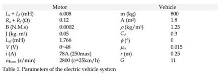
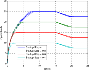
Fig. 10. Robustness test of the non-linear robust controller
0
0 10 20 30 40 50 60 70 80 90 100 time,s
Fig. 11. Performance of non-linear optimal controller
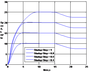
Fig. 12. Performance of double-loop PID controller
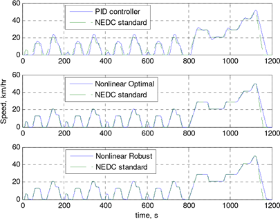
Fig. 13. Results of new European Driving Cycle test
Driven by brushless DC motor
BLDC motor is a closed loop system in nature. The back EMF introduces a negative feedback signal proportional to the motor speed, which enhances the damping of the system. Assume all the initial conditions are zero, the Laplace transform of (7) is:
Therefore, the dynamic model of an EV driven by BLDC can be obtained as shown in Fig. 14.
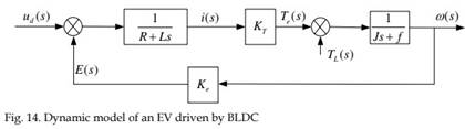
The transfer function of the inverter can be given as:
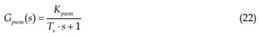
Where, Kpwm: gain of inverter; TS: time constant of PWM controller.
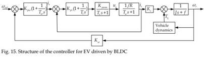
The controller of a BLDC is generally composed of current regulation loop and speed regulation loop. In practical systems, due to the fact that the electromagnetic time constant is smaller than electromechanical time constant, current regulation is faster than speed regulation. Hence, speed regulation is faster than the variation of back EMF. Therefore, the effect of back EMF on current regulation loop can be neglected. In order to have small overshoot and good tracking performance, current regulation should be designed as type-I system. Since there are two inertia elements, the current regulator should be designed as PI regulator, whose transfer function is
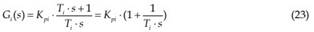
Where, Kpi: the proportional coefficient of current regulator; Ti: time constant of current regulator.
The structure of the current regulator is shown as the internal loop in Fig. 15. Negnecting the effect of back EMF on the current regulation loop, the stator circuit of the motor can be approximated as a first-order inertia element, hence:
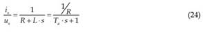
Where, Ta = L/R.
The structure of the speed regulation is shown as the external loop in Fig. 15 (Wu et al., 2005). The speed regulation system should have no steady error at steady state and good anti-disturbance capability at transient state, the speed regulator should be designed as type-II system. The speed regulation loop is composed of an integration element and an inertia element, a PI regulator should be used, leading to a transfer function
Where, Kpw: proportional coefficient of speed regulator; Tw: time constant of speed regulator.
Driven by PMSM
When designing a controller for PMSM motor, generally two control strategies, i.e., vector control and direct torque control (DTC), are used. In DTC, Stator flux linkage is estimated by integrating the stator voltages. Torque is estimated as a cross product of estimated stator flux linkage vector and measured motor current vector. The estimated flux magnitude and torque are then compared with their reference values. If either the estimated flux or torque deviates from the reference more than allowed tolerance, the transistors of the variable frequency drive are turned off and on in such a way that the flux and torque will return in their tolerance bands as fast as possible. Thus direct torque control is one form of the hysteresis or bang-bang control. In vector control, the stator phase currents are measured and converted into a corresponding complex (space) vector. This current vector is then transformed to a coordinate system rotating with the rotor of the machine. The position can then be obtained by integrating the speed. Then the rotor flux linkage vector is estimated by multiplying the stator current vector with magnetizing inductance Lm and low-pass filtering the result with the rotor no-load time constant Lr/Rr, that is, the ratio of the rotor inductance to rotor resistance. Using this rotor flux linkage vector the stator current vector is further transformed into a coordinate system where the real x-axis is aligned with the rotor flux linkage vector. The real x-axis component of the stator current vector in this rotor flux oriented coordinate system can be used to control the rotor flux linkage and the imaginary y-axis component can be used to control the motor torque.
In DTC, the switching speed is low, and the controlled motor generally has low inductance. Therefore, significant current and torque ripples are observed at low speed, limiting the speed regulation range of the controlled system. While the vector control can handle such problems very well (Liu et al., 2004). No matter under low-speed or high-speed condition, the motor current can respond very well once the current waveform required for certain rotation speed is given. The q-axis component of the current is proportional to the torque component needed, giving an excellent performance in dynamic response. Although the vector control algorithm is more complicated than the DTC, the algorithm is not needed to be calculated as frequently as the DTC algorithm. Also the current sensors need not be the best in the market. Thus the cost of the processor and other control hardware is lower making it suitable for applications where the ultimate performance of DTC is not required (Telford et al., 2000). Therefore, vector control is selected in the EV control.
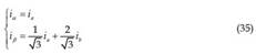
When the number of poles is fixed, the torque of a PMSM is determined by the stator current, therefore, the control of the motor is to control the current. Generally, the stator current is is first decomposed in the d-q cordinate, in which d-axis is aligned with the rotor flux and the q-axis is vertical to d-axis.

After such decomposition, is can be represented as shown in Fig. 16.
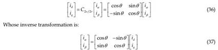
It is shown that the stator current is decomposed along the rotor axis id component and vertical to the rotor axis iq component. Then the control of the motor become the calculation of the instantaneous rotor position, i.e., the ε as shown in Fig. 16. the parameter ε can be obtained through sensor. Using an intermediate coordinate system α, β and its phase current projections i and iβ, and the fact that ia + ib + ic = 0 , one obtains:
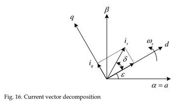
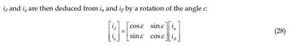
id and iq are then deduced from i and iβ by a rotation of the angle ε:
With proper coordinate transformation, the electric torque of a synchronous motor is described as follows:

Where, Φ : flux linkage.
It is shown that, for a magnetically isotropous machine the motor torque depends only on the quadrature q current component (torque component). When δ=π/ 2 (i.e., id = 0), the optimal mode of operation is achieved, where the motor produces the maximum torque.
Currently, vector control (or FOC) is an effective method in variable frequency speed regulation system in synchronous motors. It can obtain large instantaneous speed regulation range. The stator current is measured, then transformed to rotor coordinate with coordinate transformation, forming a current feedback, which can dynamically follow the variation of the current. The speed and rotor position are obtained by optical encoder, forming the speed loop, and finally implement the control of current and speed, greatly enchancing the stability, response speed and control accuracy of the system.
The key to control of PMSM is the realization of high-performance control of motor instantaneous torque. The requirements of torque control for PMSM can be summarized as fast response, high accuracy, low ripple, high efficiency and high power factor, etc. There are three regular methods in current control (Liu et al., 2009): 1) id = 0 control; 2) maximum torque and current control; 3) id < 0 field weakening control. Other methods such as constant flux linkage control or torque linear control are too complex to use.
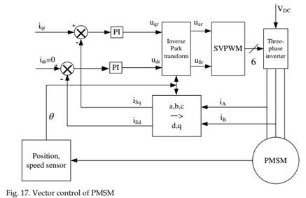
id = 0 control is simple to implement, and the EM torque and the stator current have a linear relationship, hence having no demagnetizing effect. The disadvantages of this method is the high stator voltage and low power factor at large load conditions, hence cannot fully utilize capacity. In EV control, generally the capacity required is not very large, but it needs high overload capability and good torque response performance. Hence, id = 0 control, together with maximum torque-current ratio method, is selected as the solution in EV driven by PMSM. Under such conditions, the structure of the controller is designed as shown in Fig. 17 (Cao & Fan, 2009).
Optical encoder is installed the motor rotor, which accepts the pulse signal when the rotor is rotating. With the pulse signal, the space position θ and rotor speed ωr can be calculated. Using the transforming factor e-jθr , id and iq are obtained by performing coordinate transform from ABC-coordinate to dq-coordinate on iA, iB and iC (obtained by assuming iC = – iA – iB here). The detected id and iq are compared with the reference value idr and iqr. The error signal is used for regulation, e.g. PI regulator. The inverse Park transform is applied on the calcuated input and then generator output by looking up the table. The generated output is supplied to the three-phase inverter through SVPWM (Space Vector PWM), which controls the motor.
In the SVPWM modulation system, the gain of the inverter can be expressed as:
Where, U0: DC voltage input to the inverter; UΔ: amplitude of the triangular modulation signal.
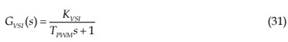
The control object of current loop is the DC-AC inverter and the stator circuit of the PMSM motor. DC-AC inverter can generally be regarded as a first-order inertia element with time constant TPWM ![]() where fΔ: frequency of the triangular modulation signal). The transfer function is:
where fΔ: frequency of the triangular modulation signal). The transfer function is:
With similar discussion in BLDC motor, the stator circuit of the motor is approximated by a first-order inertia element. Introducing a PI regulator, the system is tuned to be type-I element. The PI regulators used for d-axis and q-axis are the same, and the transfer function is:
PIi = KPi(1+ ![]() 1 ) (32)
1 ) (32)
T sii
In this case, the structure of the current regulation system is shown as the internal loop in Fig. 18. The close loop transfer function of the current regulation system can be simplified as a first-order inertia element:
![]() G sci( ) = 1+GGoi( )ois( )s = sK+ iki = sKi1+ 1 (33)
G sci( ) = 1+GGoi( )ois( )s = sK+ iki = sKi1+ 1 (33)
![]() K Kpi VSI =ωc ; ωc : close-loop bandwidth of current loop.
K Kpi VSI =ωc ; ωc : close-loop bandwidth of current loop.
Where, Ki =
T Ra s
Hence, if a PI regulator is used for speed loop, with transfer function:
Gas( )s = Ks(1+ ![]() 1 ) (34)
1 ) (34)
T ss
Where, Ks, Ts: amplification coefficient and time constant of PI regulator respectively. Then the overall model of control system is shown in Fig. 18, with the outer loop being the speed loop (Brandstetter et al., 2008).
Driven by inductor motor
Generally, VVVF based on steady motor model, DTC and vector control are used for the speed regulation for induction motor applications. The first method does not consider the complex dynamics inside the electric machine, therefore cannot achieve good dynamic performance. With DTC, although it is not affected by the motor parameters, over-current may occur due to the fact that there is no current feedback. Under low speed condition, the stator flux linkage is circular, and the current is close to sinusoidal. However, at high speed condition, the current waveform is irregular. Large harmonic currents and electromagnetic noises can be observed. Vector control, completely solved above issues. With vector control, the control of AC induction motors is as simple as that of DC motor (Sun & Li, 2002).
The basic principle of vector control is that the magnetic force and power are invariant under normal transform. First transform the model under A-B-C coordinate to α−β steady coordinate (Clarke transform), then apply Park transform to the model under α−β steady coordinate to d-q rotating coordinate.
Assume the windings of three phase A, B and C are symmetrical, and flowing through balanced sinusoidal current. Then the resultant magnetic force F is rotating with synchronous speed ϖl .
Assume balanced three phase, the projection that modifies the three phase system into the (α,β) two dimension orthogonal system is (refer to Fig. 16):
The (α,β)→(d,q) projection (Park transformation) is the most important transformation in the vector control. This projection modifies a two phase orthogonal system (α,β) in the d,q rotating reference frame. If we consider the d axis aligned with the rotor flux, for the current vector, the relationship from the two reference frame:
The model of a three-phase induction model under d-q two-axis coordinate can be expressed as follows. Votlage equations:
Flux linkage equations:
With these transformations, the stator current is decomposed into two DC components aligned with rotor magnetic field, id and iq, with id corresponding to excitation current and iq corresponding to torque current. These two currents can be controlled separately. Control of id means control the flux, while control of iq means control of torque, which is like the control of a DC motor, and then different control strategies can be easily applied on the control of EV driven by induction motor. With vector control scheme, the structure of whole system can be given as shown in Fig. 19.
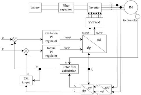
Fig. 19. The control system of EV driven by induction motor with vector control scheme
Implementation of electric vehicle controller with DSP
As the development of the high computing capability microprocessor, such as DSP (Digital Signal Processor), it is possible to perform advanced control strategies on the electric vehicle and integrate complex functions to achieve optimal performance (Huang et al., 2007). These capabilities can be utilized to enhance the performance and safety of individual vehicles as well as to operate vehicles in formations for specific purposes (Huang et al., 2007). In this section, the design and implementation of an EV controller with DSP will be discussed.
An EV controller may preferably have following functions:
• Due to the frequent acceleration/deceleration and up/down of EV, it is preferably that the regenerative control function is included, to save energy in battery and hence enhance the driving range per charge;
• Self diagnostics and restoration from failure;
• Scalable to function expansion;
• And comprehensive protection functions, including over-temperature protection, overvoltage and under-voltage protection, over-current protection, short-circuit protection, motor-lock protection, and protection for control unit, main switch and security, etc.
Fig. 20 shows detailed implementation of a EV controller with DSP (Huang et al., 2007). The whole system is composed of power circuit and control circuit. The control circuit include two parts. One is the external control circuit including auxiliary power supply, MOSFET driving circuit, isolation & protection circuit and contactor driving circuit. These circuits have common ground with the battery group. Another one is the kernel control circuit, including DSP kernel TMS320F2812, variant protection circuits, detection circuit, signal conditioning circuit, CAN communication circuit, external watchdog circuit and isolated auxiliary power system, etc.
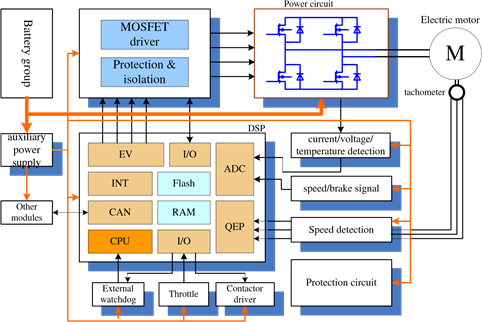
Fig. 20. Structure of a DSP-based EV controller
The control flow of the whole system, as shown in Fig. 20, is that the DSP generate PWM modulation signal, which is used to drive the power converter (chopper for DC motor and inverter for AC motor) after isolation and amplification. The power converter controls output of the battery to control the speed of the motor, and implement the energy regenerative control. The voltage, current and speed signal of motor are detected and sent to DSP after signal conditioning, to form a feedback control.
The control circuit detects the voltage, current, temperature and rotation speed to realize the function of regulation and protection, and provides support for implementation of advanced control strategies. The voltage, current, and temperature are measured through the quantification of AD converter in DSP kernel. The speed is detected with the QEP (quadrature encoder pulse) inside the DSP, and the speed signal is used for realization of loss-of-control protection, smooth startup control, anti-skip control during up-hill startup and providing speed information for the driver. Speed regulation (throttle) and breaking signal are generated by proper device and acquisited by AD of the DSP after signal conditioning.
The gear shift is digital signal. It is input to the DSP through I/O after isolation and amplitude limiting. The main contactor is connected in series with the power circuit. The winding of the contactor is controled by digital signal output from the I/O of DSP, to switch on or off the power circuit. In order to restore the whole system from severe failure, double watchdog (internal and external) is used. When the DSP is invalidated, the external watchdog can reset the chip to restore the normal operation of the controller. Even the DSP chip is destroyed, the output of the controller is switched off due to the continuing resetting. With this scheme, the security of the EV is assured even under severe failure in the controller.
The power converter is controlled by PWM, which is generated by two event managers (with one generating 16 PWM signals). The PWM’s generated by the event managers of DSP are sent to drive the power converter after isolation and amplification. When there are faults in the power converter or in driving circuit, the fault information is sent to DSP through its I/O after isolation.
The configuration of controller parameters, various state information and fault information are exchanged with external devices, such as portable computer, handheld programable devices, or display monitor on the EV, through CAN (controller area network) bus, which is controlled by the embedded CAN controller in DSP.
The power converter is composed of semiconductor power electronics devices and their snubber circuit and freewheeling diodes. Power semiconductor is the key for power conversion in EV controller. Now, new generation of power semiconductor devices are developed and the performances are improved continuously. Presently, in most of EV control applications, MOSFET (metal–oxide–semiconductor field-effect transistor) or IGBT (insulated-gate field-effect transistor) is used. IGBT needs higher driving power, but has lower working frequency. MOSFET has the advantage of simple driving circuit and low conducting resistance, making it specially suitable for driving application in high-current low-voltage motor. In this chapter, the results are all based on MOSFET.
The main flow chart of the software running inside the DSP processor is shown in Fig. 21. It is a state-based processing system, in which the status of the whole EV system is detected in a real-time manner, various functions are activated once certain failure is detected or specific order is received. The maximum delay of processing different failure is one main-loop processing cycle.
Fig. 22 is the test platform in laboratory, in which the load torque is a brake dynamometer. Shown in Fig. 23 and Fig. 24 are the performance of regenerative braking and speed regulation with a PMSM motor.
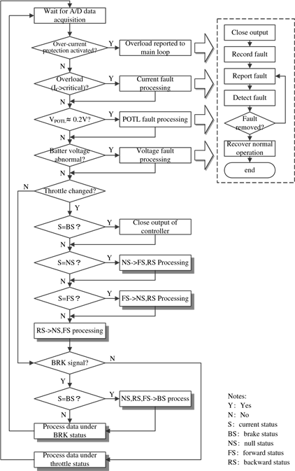
Fig. 21. Operation of the EV controller
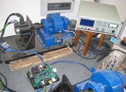
Fig. 22. Test platform of controller
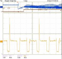
Fig. 23. Waveform of battery charging current under regenerative braking
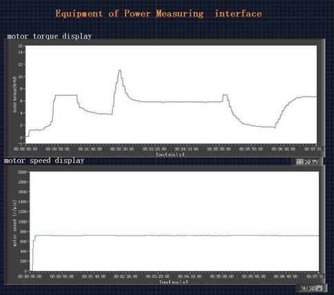
Fig. 24. Performance test of speed control of the designed controller
Conclusion
In this chapter, the modeling of electric vehicle is discussed in detail. Then, the control of electric vehicle driven by different motors is discussed. Both brushed and brushless DC (Direct Current) motors are discussed. And for AC (Alternative Current) motors, the discussion is focused on induction motor and permanent magnet synchronous motor. The design of controllers for different motor-driven electric vehicle is discussed in-depth, and the tested high-performance control strategies for different motors are presented. The model-based controller is designed for brushed DC motor, while for other motors, model based controllers can be designed in a similar way if the control strategies discussed in this chapter are used. Finally, the implementation of the controller with DSP and some test results with this platform are presented.