The damages and loses caused by earthquakes are increased as urbanization increased in past decades. However, scientists currently cannot predict the time, location and magnitude of an earthquake accurately. Currently, the earthquake predictions are not yet reliable, so long-term probabilistic earthquake hazard analysis and rapid post-earthquake early warning are two alternative solutions to reduce potential earthquake damages [1-3].
For long-term ground motion forecasts, seismic hazard maps are widely used for estimating probabilities of ground motion exceeding certain amount in different areas in 50 years. In addition, the ground motion estimations in seismic hazard maps are useful for different applications, including, for instance, building codes, insurance rates, land-use policies and education of earthquake response. In United States, the U.S. Geological Survey (USGS) periodically updates the National Seismic Hazard maps that provide a 50 years ground motion estimations for United States[4, 3]. To consider effects form different aspects, the National Seismic Hazard maps incorporate both geological and geophysical information in ground motion estimations[3]. Recent advances in computational seismology allow us to simulate wave propagation in complex velocity structure models and then open the probability of physics-based long-term ground motion estimations. The Southern California Earthquake Center (SCEC) has developed a methodology which considers both source and structure effects in ground motion simulations for long-term ground motion estimations in Los Angles region[5].
The earthquake early warning systems are designed for short-term ground motion forecasts. The idea of earthquake early warning systems is based on the transmission speed of electromagnetic signal is much faster than the propagation speed of seismic shear-waves and surface waves that usually generate strong ground motion [2]. The Earthquake Alarms Systems, ElarmS, is the earthquake early warning systems designed for California region [1, 2]. The ElarmS uses the signal of the first arrived primary waves to estimate magnitudes, locations and then estimate peak ground motions of earthquakes [1, 2]. Here we propose a rapid full-wave Centroid Moment Tensor (CMT) inversion method for earthquakes in Southern California [6]. The algorithm has potential for (near) real time CMT inversion and then use optimal CMT solutions to generate peak ground motion maps for earthquake early warning purposes. In addition, the full-wave ground motion forecasts, which include basin amplification effects, source effects and wave propagation effects in the 3D structure model, will provide more accurate and detailed estimations.
USGS National Seismic Hazard Maps
In the United States, the USGS incorporates different geophysics and geological information to continually update the National Seismic Hazard Maps for log-term ground motion forecasts[4, 3]. In USGS hazard maps, source models, including seismicity models and faults source models, and attenuation relations are two main components[3]. The Southern California is included in the western U.S. hazard maps, so here we take western U.S. as an example for explaining the procedures of hazard maps of USGS.
To estimate potential seismicity, we need to consider earthquake recurrence in or near the locations of past earthquakes occurred and the possibility of earthquake occurrences in areas never have earthquakes. First, the gridded-seismicity models are based on earthquake catalogs and historical earthquakes. The seismicity rates in each grid (0.1° longitude by 0.1° latitude) are based on the number of earthquake in it [3]. To smooth the seismicity rates, a 2D Gaussian function is applied to the model[3]. In most of areas the correlation distance is 50 kilometers, but in high seismicity regions the correlation distances parallel to the seismicity trends is 75 kilometers and normal to the seismicity trend is 10 kilometers to avoid effecting the seismicity estimations near the fault zones[3]. The uniform background seismicity models are used to estimate the possibilities of random earthquakes in aseismic regions [3]. The western U.S. region is separated into few sub-regions and the uniform background seismicity rate in each sub-region is based on the annual seismicity rates of earthquakes with Mw ≥ 4 since 1963 [3]. Now, there are two seismicity rate estimations in each grid cell. If the uniform background seismicity rate is larger than the gridded-seismicity rate in a grid, the final seismicity rate is the sum of 67% gridded-seismicity rate and 33% of uniform background seismicity rate in that grid; otherwise, the final seismicity rate just equals to the gridded-seismicity rate in the grid [3].
Existing fault zones have relative high possibilities of occurring destructive earthquakes. The fault source models are based on geological fault studies, geodesy and seismological date to estimate geometries, maximum magnitudes and recurrence periods for fault zones [3, 7]. To obtain fault geometries, the geological surveys and earthquake location distributions are used for estimating fault areas. The maximum magnitudes in fault zones could be inferred from relationships between fault areas and magnitudes or historical magnitudes [3, 7]. The Gutenberg-Richter magnitude-frequency distribution and the characteristic rate on a fault, ratio of the slip rate to the slip of the characteristic earthquake of the fault, are used in earthquake recurrence estimations [3]. In California region, USGS gives 67% on the characteristic rate and 33% on the Gutenberg-Richter [3]. The Uniform California Earthquake Rupture Forecast, Version 2 (UCERF 2) [7] presented in 2007 Working Group on California Earthquake Probabilities (WGCEP) is used as the fault source model in California region. In seismic hazard maps, fault sources only consider type-A faults that have information on fault geometries, slip rates and earthquake data and type-B faults that only have information on fault geometries and slip rates[3].
In California region, the gridded-seismicity model is derived form earthquake catalog and estimates probabilities of earthquakes between Mw 5 to 7.0 [3]. In addition, the fault models also estimate the possibilities of earthquakes with Mw larger than 6.5 to consider the possibilities of destructive earthquakes in fault zones [3]. When the two types of source models are put into seismic hazard maps the probabilities of earthquakes between Mw 6.5 to 7.0 may over estimated. For more accurate estimations, the seismicity rates of Mw ≥ 6.5 in gridded-seismicity model reduced by one-thirds in fault zones [3].
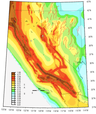
FIGURE 1.
The California seismic hazard map of 1 Hz spectral acceleration (SA) for 2% exceedance probability in 50 years. Adopted from [3].
The Next Generation Attenuation (NGA) database developed by Pacific Earthquake Engineering Research Center (PEER) is used in USGS hazard maps as attenuation relations for ground motion predictions[8, 9, 3]. The NGA database is not only an empirical ground motion model derived from selected recordings but also includes 1D ground motion simulations, 1D site response, and 3D basin response results from other studies [8]. So, the database includes many essential effects, including, for example, basin response, site response, earthquake rupture properties and style of faulting.
Hazard curves, exceedance probability as a function of ground motion, are derived from source models and attenuation relations of grids. The final seismic hazard maps are made by interpolating annual exceedance probabilities form hazard curves in the model. On the California 1 Hz spectral acceleration (SA) hazard map [Figure 1], high hazard level regions are controlled by the major faults in California.
A Physics-based seismic hazard model: CyberShake
The CyberShake, one of the Southern California Earthquake Center’s (SCEC) projects, is a seismic hazard model that uses full-wave method to simulate ground motions in Southern California. Here the term “full-wave” means using numerical solutions to compute the exact wave equation, rather than approximations. Recent advances in computational technology and numerical methods allow us to accurately simulate wave propagations in 3D strongly heterogeneous media [10, 11], and opened up the possibility of simulation-based seismic hazard models [5],extracting more information from waveform recordings for seismic imaging [12-14] and earthquake source inversions [15, 6]. For seismic hazard model, these physics-based simulations consider factors that affect ground motion results, for example, source rupture and wave propagation effects in a 3D velocity structure and then provide more accurate ground motion estimations.
The Los Angeles region is one of the most populous cities in the United States. The city is in a basin region and near active fault systems, so a reliable seismic hazard model is important for the city. The CyberShake selected 250 sites and simulated potential earthquake ruptures in Los Angeles region to build a seismic hazard model [5]. The SCEC Community Velocity Model, Version 4 (CVM4) which has detailed basins and other structures is used as the 3D velocity model in simulations [16].
The potential earthquake ruptures within 200km and Mw larger than 6.0 in the Los Angeles region are selected from the Uniform California Earthquake Rupture Forecast, Version 2 (UCERF 2) for ground motion simulations in Cybershake [5]. The earthquake ruptures in UCERF2 only provide possible magnitudes in faults, without information of rupture process. To consider the earthquake rupture effects, each earthquake rupture selected from UCERF2 could convert to a kinematic rupture description for numerical simulations [5] based on Somerville et al.’s method [17].
In CyberShake, ground motion predictions are based on physics-based simulations rather than empirical attenuation relations. The qualified rupture sources are more than 10,000 in the Los Angeles region [5]. However, when the uncertainties of earthquake ruptures are considered, the number of earthquake rupture increases to more than 415,000. It will take a lot of computational resources and time to simulate all rupture models [5]. An efficient method is storing receiver Green’s tensors (RGTs) of selected sites in the model and applying reciprocity to generate synthetic seismograms of rupture models [18, 5]. The RGTs called strain Green’s tensors (SGTs) in CyberShake project [5]. Following Zhao et al. [18], the displacement field from a point source located at r’ with moment tensor Mij can be expressed as [19]

where ∂j’∂j’denotes the source-coordinate gradient with respect to r’r’ and the Green’s tensorGki(r,t;r’)Gki(r,t;r’)relates a unit impulsive force acting at location r’r’ in direction Unexpected text node: ‘e ‘Unexpected text node: ‘e ‘to the displacement response at location r in directionUnexpected text node: ‘e ‘Unexpected text node: ‘e ‘. Taking into account the symmetry of the moment tensor, we also have

Applying reciprocity of the Green’s tensor

equation (2) can be written as

For a given receiver location r = rR, the receiver Green tensor (RGT or SGT) is a 3rd-order tensor defined as the spatial-temporal strain field

Using this definition, the displacement recorded at receiver location rR due to a source at rS with moment tensor M can be expressed as

and the synthetic seismogram due to a source at rS with the basis moment tensor Mm can be expressed as

In CyberShake, the SGTs can therefore be computed through wave-propagation simulations of two orthogonal horizontal components with a unit impulsive force acting at the receiver location rR and pointing in the direction e^k in each simulation and store the strain fields at all spatial grid points r’ and all time sample t. The synthetic seismogram at the receiver due to any point source located within the modeling domain can be obtained by retrieving the strain Green’s tensor at the source location from the SGT volume and then applying equation (6).
In CyberShake project, one of objectives is improving the Ground Motion Prediction Equations (GMPEs), which are widely used in seismic hazard analysis, by replacing empirical ground motion database with physics-based simulated ground motions. Some advantages in physics-based simulation results could be found by comparing hazard curves among different methods. The hazard curves derived from Boore and Atkinson’s [20] method and Campbell and Bozorgnia’s [8] method that consider basin effects in GMPEs are selected for comparisons. However, the earthquake rupture directivity effects are not considered in these methods.
Here, three hazard curves which show exceedance probability for spectral acceleration (SA) at 3 seconds period are used to discuss differences among results [Figure 2]. At the PAS site [Figure 2], a rock site, the hazard curves among the three methods are similar. At the STNI site [Figure 2], a basin site, the hazard curves of CyberShake and Campbell and Bozorgnia’s [Figure 2] method which consider basin amplification effects are similar, but the hazard curve of Boore and Atkinson’s [20] method is significantly lower than the other two curves. However, at WNGC site, the hazard curve of CyberShake has higher hazard level than the other two. The WNGC site is at the region that channeling energy from earthquake ruptures in the southern San Andreas fault into Los Angeles basin, and the factors are included in physics-based simulations. The channeling phenomenon also can be found from other studies [21, 22]. The CyberShake seismic hazard map [Figure 3] is derived from the 250 sites used in simulations [5]. In the physics-based hazard map, some effects don’t include in attenuation relations, including, for example, earthquake rupture effects, basin amplification effects, and wave propagation phenomena in 3D complex structures.
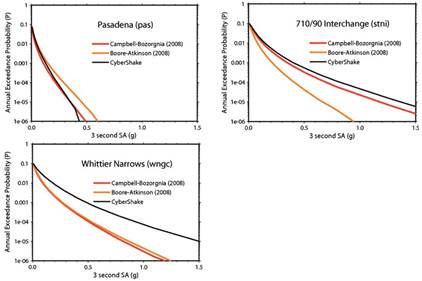
FIGURE 2.
Hazard curves derived form three different methods at three sites, PAS, STNI and WNGC, in Los Angeles region. The red lines represent the results of using Campbell and Bozorgnia’s [8] method; the orange lines represent the results of Boore and Atkinson’s [20] method; the black lines represent the results of CyberShake. Adopted from [5].
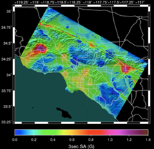
FIGURE 3.
The CyberShake hazard map for Los Angeles region of 3 seconds period spectral acceleration (SA) for 2% exceedance probability in 50 years. Adopted from [5].
Comparisons between USGS and CyberShake hazard maps
There are many differences between the hazard maps of USGS and CyberShake, including, procedures of making hazard maps, required computational resources and results [3, 5]. The USGS National Seismic Hazard maps in California region are derived form source models based on seismological data, geological surveys and earthquake rupture models, and the Next Generation Attenuation (NGA) database [8, 9]. The CyberShake hazard map is constructed by physics-based simulations in the 3D velocity model for all potential earthquake ruptures with Mw ≥ 6.0 near Los Angeles region [5]. The computational resources requirements for generating USGS hazard maps do not mention in the 2008 report of seismic hazard maps update, but the hazard maps should be able to done without a super computer. To generate the CyberShake hazard map, lots of wave propagation simulations are required to build a database for generating synthetic seismograms of potential earthquake ruptures [5]. The computational resource of physics-based seismic hazard maps is much higher than the computational requirement of USGS hazard maps. However, the advances in computer sciences make the computational requirements affordable for CyberShake, also accurate estimations of ground motions are important for a city with a large population. The seismic hazard levels are quit different in the Los Angeles region between two hazard maps. In the USGS hazard map [Figure 1], the high hazard level regions are almost along the fault zones and hazard values decrease as the distance between a site and fault zones increases. In the Los Angeles basin region, the hazard level is about the same in the USGS hazard map [Figure 1]. In the CyberShake hazard map, the hazard values along the San Andreas fault are high, but the width of high hazard zones is narrower. In addition, the CyberShake hazard map in the Los Angeles basin has more details [5]. This probably reflects the source and structure effects in ground motion predictions.
ElarmS: Earthquake alarms systems for California
In Southern California, an earthquake-prone area, many cities are under earthquake risks, hence earthquake early warning systems are becoming an important role in earthquake disaster mitigation [2]. Allen [2] developed earthquake early warning systems called Earthquake Alarms Systems (ElarmS) for California. In the ElarmS methodology, three steps are designed for rapid estimations of earthquake source parameters and prediction of peak ground motions [1, 2]. First, using the time information of first-arrived signal to locate earthquakes and estimate the warning time. Second, using frequency information of first four seconds of P-wave to estimate magnitudes of earthquakes. Third, using attenuation relations and the earthquake source information, an estimated location and magnitude, to generate ground shaking maps.
In the ElarmS, the arrival times of P-waves are used to rapidly locate earthquake locations. The possible areas of an earthquake location could be inferred by using the information of the first two or three stations trigged by an earthquake. To locate a more accurate earthquake location, including, longitude, latitude, depth and origin time, the first arrival time form four stations are required. A grid search algorithm is used to find an optimal earthquake location that has minimum arrival time misfits. The warning time, the remaining time before the peak ground motion arrived, can be estimated by using the predicted S-wave arrival times of sites. Peak ground motions are usually caused by S-wave or surface wave, so use predicted S-wave arrival times as peak ground motion times may provide additional warning time for some sites.
The magnitude, which represents the released energy of an earthquake, is an important parameter in earthquake early warning systems. The rapid magnitude estimation method of an earthquake by using the frequency information of the first four seconds of P-wave is adopted in the ElarmS [1, 2]. Basically, the magnitude estimations take two procedures. The first step is finding the maximum predominant period within the first 4 seconds of the vertical component P-wave waveforms, and then use linear relations to scale the maximum predominant period value to an estimated earthquake magnitude [1, 2]. As the number of the maximum predominant period value from different receivers increases, the average magnitude errors will decrease [2].
When the location and magnitude of an earthquake is available, attenuation relations can be used to estimate ground motions of sites and then generate a ground motion prediction map for whole California. In the ElarmS, the attenuation relations are based on the recordings of earthquakes with magnitude larger than 3.0 in California [2]. However, the empirical attenuation relations used in the ElarmS do not account effects of wave propagation in 3D structures, for example, basin amplification effects.
Rapid full-wave CMT inversion
In Southern California, preliminary 3D earth structure models are already available, and efficient numerical methods have been developed for 3D anelastic wave-propagation simulations. We develop an algorithm to utilize these capabilities for rapid full-wave centroid moment tensor (CMT) inversions. The procedure relies on the use of receiver Green tensors (RGTs), the spatial-temporal displacements produced by the three orthogonal unit impulsive point forces acting at the receivers. Once we have source parameters of earthquakes, a near-real time full-wave ground motion map, that considers both source and wave-propagation effects in a 3D structure model, may also available for earthquake early warning purposes.
In our CMT inversion algorithm, the RGTs are computed in our updated 3D seismic structure model for Southern California using the full-wave method that allows us to account for 3D path effects in our source inversion. The efficiency of forward synthetic calculations could be improved by storing RGTs and using reciprocity between stations and any spatial grid point in our model. In our current model, we will use three component broadband waveforms below 0.2 Hz to invert source parameters. Based on Kikuchi and Kanamori’s [23]source inversion method, any moment tensor can be expressed as linear combination of 6 elementary moment tensors. In our current coordinate (x=east, y=north, z=up), the moment tensor can be expressed as below:

There are two main advantages of using this method. First, different subsets of 6 elementary moment tensors could represent different source parameter assumptions such as M1~M6 could recover general moment tensors and M1~M5 could represent pure-deviatoric moment tensors [23]. From efficiency point of view, we only need to generate synthetic waveforms of 6 elementary moment tensors at grid points close to initial sources locations for receivers to invert an optimal CMT solution.
For centroid locationx1x1 and centroid time t1, the synthetic seismograms of 6 elementary moment tensors could be defined as:

where r is receiver, m is index of 6 moment tensor, i is component index. The synthetic seismogram can be expressed as:

From inversion point of view, the phases have less structure heterogeneous effects can reduce the nonlinear effects caused by complex 3D structure such as body wave phases that propagate through relative simple deep structure and surface wave phases that propagate along free surface and average out the heterogeneity. We apply our seismic waveform segmentation algorithm that is based on continuous wavelet transforms and a topological watershed method to observed seismograms and then select the first (potential body wave) and biggest (potential surface wave) time-localized waveforms to invert source parameters.
In source inversion, we applied a multi-scale grid-searching algorithm based on Bayesian inference to find an optimal solution [Figure 4]. We consider a random vector H composed of 6 source parameters: the longitude, latitude and depth of the centroid location rS, and the strike, dip and rake of the focal mechanism. We assume a uniform prior probability P0(H) over a sample space Ω0, which is defined as a sub-grid in our modeling volume centered around the initial hypocenter location provided by the seismic network with grid spacing in three orthogonal directions given by a vector θ0 and a focal mechanism space with the ranges given by 0°≤ strike ≤360°, 0°≤ dip ≤90° and -90°≤ rake ≤90° and with angular intervals in strike, dip and rake specified by a vector0.
We apply Bayesian inference in three steps sequentially. In the first step, the likelihood function is defined in terms of waveform similarity between synthetic and observed seismograms. We quantify waveform similarity using a normalized correlation coefficient (NCC) defined as

where n is the observation index, sn¯¯¯(t) and sn(t) are the filtered observed seismogram and the corresponding synthetic seismogram, [t0n,t1n][tn0,tn1]is the time window for selecting a certain phase on the seismograms for cross-correlation (Figure 4b). We allow a certain time-shift ΔtΔt between the observed and synthetic waveforms. To prevent possible cycle-skipping errors, we restrict |Δt||Δt| to be less than half of the shortest period. We assume a truncated exponential distribution for the conditional probability

where λn is the decay rate. Assuming the NCC observations are independent, the likelihood function can be expressed as

where N is the total number of NCC observations. The posterior probability for the first step can then be expressed as

Where

We note that the λnλn in front of (1-NCCn) in equation (14) can be used as a weighting factor for various purposes, such as to account for different signal-to-noise ratios in observed seismograms and to avoid the solution to be dominated by a cluster of closely spaced seismic stations.
The probability for individual measurements

can be used for rejecting problematic observations. In practice, we only accept observations with

A very lowP0(NCCn) indicates that the nth observed waveform cannot be fit well by any solutions in our sample space. This may be due to instrumentation problems or unusually high noise levels in the observed waveform data.
In the second step, we apply the same algorithm on another measurements, time-shifts between the observed and synthetic waveforms when the NCC is the maximum in allowed time-shift range. The last step is applying the same processes to the amplitude ratio measurements. By using the Bayesian approach, we can obtain the probability density functions of source parameters that contain uncertainties information rather than a single best solution. Our optimal source parameter solution is the one with highest probability. In Figure 4, examples of the marginal probabilities for some of the source parameters are shown for the 3 September 2002 Yorba Linda earthquake.
For earthquake early warning purposes, there are few approaches to make our CMT inversion method toward (near) real time and then use optimal CMTs for generating full-wave peak ground motion maps. To save some time in generating synthetic seismograms, we can store synthetic seismograms of 6 elementary moment tensors rather than extract them from RGTs. Destructive or larger earthquakes tend to occur in existing fault zones or regions where earthquakes occurred. Based on the assumption above, rather than store synthetic seismograms of all grid points in our model, we can store the synthetic seismograms of grid points near fault zones or high seismicity regions. Another possibility is to save time of inversion by using other efficient inversion algorithms. Full-wave ground motion prediction maps could be generated based on the synthetic seismograms of optimal CMT solutions.
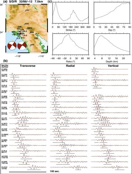
FIGURE 4.
An example of our CMT inversion procedure. (a) The map shows epicenter of the 3 September 2002 Mw 4.3 Yorba Linda earthquake (the star), the best-fit double-couple solution (the red beachball) and stations (gray triangles) selected for this inversion. (b) Examples of the waveforms selected for in the CMT inversion. The black lines are observed seismograms and the red lines are synthetic seismograms. The black bars indicate the selected waveform segments for CMT inversion. (c) The marginal probability densities for strike, dip, rake and depth obtained after our grid-search step.
The speed of earthquake source parameters estimation and accurate ground motion predictions are both play essential role in earthquake early warning systems. In the ElarmS, earthquake locations, origin time and magnitudes could be inverted in very short time. Peak ground motion maps can be generated shortly by using empirical attenuation relations. The CMT inversion method we proposed has potential for (near) real time inversion and then solutions could be used for (near) real time full-wave peak ground motion maps. In addition, the Bayesian approach used in our CMT inversion has uncertainty of solutions and could be projected into ground motion estimations.
Conclusion
In this chapter, we compare full-wave based and non-full-wave based methods of ground motion forecast for (southern) California. There are advantages and disadvantages to different methods. Since the full-wave methods involve numerical simulations of wave propagation in 3D velocity models, the computational resource requirements are much higher than non-full-wave methods. However, numerical simulations are usually affordable in most of super computers. In general, ground motion estimations of non-full-wave methods are usually based on empirical attenuation relations. In full-wave methods, the ground motion estimations are based on numerical simulations that considered source effects, basin amplification effects and wave propagation effects in a 3D complex velocity [5, 6]. Those effects may play very important roles in ground motion estimations. For example, if a large earthquake occurs on southern San Andreas fault, the released energy will channel into Los Angeles region, one of the most populous cities in the United States, and basin effects will amplify the ground motion [22, 5]. Full-wave based ground motion forecast should able to provide more accurate and detailed ground motions and this will benefit cities under earthquake risks, such as Los Angeles city.
