Motto: „And what, I said, will be the best limit for our rulers to fix when they are considering the size of the State and the amount of territory which they are to include, and beyond which they will not go?
What limit would you propose?
I would allow the State to increase so far as is consistent with unity; that, I think, is the proper limit.” – Plátōn
As the rapid growth of world population and its concentration in cities around the globe takes place, sustainable urban development has constituted a crucial element affecting the long-term outlook of humanity (Auclair, 1997). Besides, in the urbanized areas a high level of GDP (gross domestic product) concentration can be observed. That should make us care for the operational efficiency of the urban areas more and more studiously. Dynamic and continuous horizontal and vertical growth of urban areas makes the question of efficiency more and more important. Handling productivity concentration has been a key issue for economists and solving transportation problems – due to population concentration – has been just as important for engineers for a long time. Representatives of abysmally separated scientific fields tried to solve the efficiency problems of certain areas which can be characterised by lack of capacities, extreme population and productivity density.
To effectuate an uniform, consistent methodology for urban planning – taking into consideration the viewpoints of the land use and the transportation – according to Platon’s words, we need to approach the subject by considering complex social and economic aspects. With the desire to achieve urban development that meets the needs of the present without compromising the ability of future generations to meet their needs (WCED, 1987), urban development is required to minimize threats from wasteful use of non-renewable regenerations, to avoid the uncompensated geographical or spatial displacement of environmental costs onto other places, and not to draw on the regeneration base and waste generation capacities to the levels which disrupt dynamic equilibrium of the ecosystem (Burgess, 2000).
The structure of urban areas can be understood as a result of the relationship between transport and land-use. The interaction is known as a two-way process. This process, however, is more complicated than other reciprocal processes that are frequently encountered in everyday life. This is mainly because the various interactions take place over different time scales and involve factors with varying degrees of certainty. Hence, an analysis of the interaction between transport and land-use requires disentangling diverse relationships among the factors and this makes it a difficult task.
For sustainable urban development it is inevitable to constitute policies – based on a useful planning method – that can support sustainable urban development without sacrificing either economic growth or the freedom of movement. Sustainable urban policies have to be based on comprehensive planning with the involvement of different sectors and fields of competence.
To effectuate a uniform, consistent planning methodology a flexible, consistent, and well manageable model needs to be developed, which involves the aspects both of land use and transportation. Beside this, it is important to see that planning methods generally focus on estimating and comparing the effects of one or two selected measures (e.g. infrastructure investments, land-use or fee-collection possibilities). In contrast to the above mentioned process the assignment of the best solution from a given set of measures seems to be more effective.
Based on this assumption we introduce a newly developed optimizing method. With this it is possible to describe individual system components’ (e.g. consumers, firms) behaviour, to estimate and compare social effects of the changed urban environment (based on the investigated set of measures) and furthermore to define optimal solution from a social point of view. Hereby we will have the possibility to control the urban environment based on the available set of measures (as a part of the controlling method), the object of the individual system components (energy consumption, costs, benefits – as a part of the modelling method) and the selected social objectives (e.g. operational efficiency, summed up social costs, summed up social benefits, pollution – as a part of the controlling method).
Objectives
As it was mentioned above the current method of selecting the development package comprising the most beneficial measures is to select the best measures by comparing their expected impact, after which the development strategy can be formulated based upon the joint implementation of selected measures. The effects of community development plans on the local level are often evaluated solely from a transport perspective. The state of the art, activity chain-based transport models analyse community interests with regards to mobility demand. However, this can lead to the omission of such important aspects as the use of community land in accordance with community interests.
The limiting factor that makes activity-based modelling unsuitable for the analysis of some of the aspects of community development is evident from its very definition.
The definition by Torsten Hägerstrand (Hägerstrand, 1970) states that transport decisions are induced by individual activities responsible for mobility demand. Individuals make these decisions based on changes in the utility function related to transport processes. For example, the farther a given activity is from the starting point of the trip, the less the increase in the utility function, while the comfort level associated with the mode of transport decreases the opportunity cost.
When comparing the above with the general definition of the utility function, a contradiction arises, since the definition states that utility is the property which makes things fit for the purpose of meeting individual needs. Needs inspire and energize action, while directing it at the same time (Hunyady, 2003).
Considering how transport demand is primarily generated by the fact that the production, use and consumption of products and services are separated, the dependence of transport on the demand for the original product or service cannot be ignored (Gubbins, 2003). Therefore, keeping the secondary role of transport in mind, we can come to the conclusion that demand which can be met in its entirety by transport alone rarely arises.
The enforcement of community interests, on the other hand, requires an analysis of the changes in the utility function as comprehensive as possible, since – starting from the dictionary of definitions – interest is “necessary and important, for the benefit of someone or something” (Juhász, 2003).
Taking into account that transport demand is usually not the only constituent in complex human needs, the goal of the chapter is to expand the evaluation procedure based on transport models in use today for supporting community development decisions. Analysing the changes in the utility of the individual (e. g. estimating the effects of consumed goods), the modelling of individual decisions that affect how a community works becomes possible. A further goal of the chapter is to introduce a community development process using the utility and decision theory of economics that analyses the utilization of urban areas, the structure of the transport system and the properties of the economic and social strata in a complex manner, also taking interactions between these aspects into account. Additionally the paper introduces a process to maximize social utility as a function of community development initiatives. This could be an important contribution to the development of a methodology for the selection of the urban development packages that best enforce community interests.
The model development orientations are based on the evaluation of the related literature. This approach makes it possible to analyse the model development processes and the reasons of methodological evolution. Beside this, the detailed literature analysis explains the chosen development orientations of our research.
Evolution of urban models
Before the investigation of the development process of urban models, the reasons for the evolution of the methodologies. Ambition to forecast the needs for transport can be originated from modelling of individual needs, which include physiological needs, safety, social needs, the needs for appreciation and self-realization according Maslow’s theory (Maslow, 1943). In Maslow’s hierarchy model of needs, the lowest level of necessities is the subsistence. Man always provided the goods for subsistence by production. Hence the efficiency of production directly influences the level of complacency. So it is understandable that urban models aim to represent the operation efficiency of urban system and to forecast traffic structure, which directly effects productivity.
Evolution of transport models
In modern history, the industrial revolution of the nineteenth century led to a very dynamic development on both micro and macro level. The economic growth generated by the industrial revolution coupled with the rapid expansion of transport needs generated bottlenecks in the transport system. Thus it is not surprising that the history of the modelling started in the nineteenth century. The well-known gravity model applied in transport modelling based on one of the most elemental rule of the classical physics was probably first formulated by Carey (Carey, 1873).
After the First World War the economic growth further escalated, the effect of which gave a higher priority to infrastructure development. The formulation of metropolitan areas led to the restructurization of transport needs. The main problem of the spatially concentrated urban areas became the rapid intensification of transport demand. After the Second World War the economic growth could continue, which resulted further increases in transport needs. It is not surprising that the first complex transport models, which contain the bases of the urban transport planning methodologies used nowadays, developed in 1950’s for the first time. The well-known six-step-model (data collection, forecast, goals, network proposals, testing network proposals, evaluation) was first introduced by Dr. J. Douglas Caroll in the Detroit Regional Traffic Study. The final method was worked out and applied also by Dr. J. Douglas Caroll in the Chicago Regional Transport Study (Chicago Area Transportation Study, 1962).
In the 60’s and 70’s the urbanization was gaining a bigger and bigger impetus.. For instance the population of San Francisco Bay metropolitan increased by more than 70% (ABAG, 1991) area between 1950 and 1970. This tendency reduced the applicability of traditional models, since those did not take into consideration the personal motivations of travellers and the temporal characteristics of their decisions. As a result of the demand for more effective estimation, the activity-based model of San Francisco Area was developed in the middle of seventies by Ruiter and Ben-Akiva (Ruiter & Ben-Akiva, 1978), where the econometric approach of transport planning was firstly applied in practice. Activity-based transport models are widely used by now, since those make it possible to forecast individual travel decisions more and more effectively.
Evolution of economic equilibrium models
Beside transport models, nowadays equilibrium models are also more prevalently applied in the field of urban modelling. However, their basic methodology did not contain any spatial representation until the end of the 20th century.
Most of the microeconomic models are prepared according general equilibrium conditions. The intellectual roots of the assumption of the self-regulating nature of markets – the formation of the economic equilibrium – can be originated from the so called “Invisible hand” theory of Adam Smith (Smith, 1776). The concept of general equilibrium – according to the apt statement of János Kornai – plays a similar role in the economics as the absolute-zero in the physics, which cannot be obtained in the real life, but is well defined in theory. It can be defined as an abstract point of reference. Real economic systems can be characterized by the distance they are away from the theoretical equilibrium point (Kornai, 1971).
The evolution of equilibrium theory continued in the second half of 19th century. In 1874, Léon Walras in the “Elements of Pure Political Economics” (Walras, 1871) laid down the foundations of equilibrium analysis. Walras assumes the economy to consist of households and firms. Both consumers and firms take prices as given, and market decisions depend on the equilibrium price. Each household owns resources and products applicable for final or intermediate consumption. Households gain income from the sale of resources.
After his retirement, in 1892, Walras was followed by Vilfredo Pareto in his chair as the head of the Department of Political Economics at Academy of Lausanne. Thanks to his work, general equilibrium theory’s applicability in practice was greatly improved by “Pareto optimum” (Pareto, 1897). The “Pareto optimum” is not simply one of the possible market equilibriums, but the equilibrium, in case of which none of the actors can increase their utility, without declining the utility of another actor.
In the 20th century, among others for instance Paul Samuelson investigated the dynamic stability of the equilibrium models applying the methodology of mathematical statistics (Samuelson, 1941). Dixit and Stiglitz published their theory on “The “Monopolistic Competition and Optimum Product Diversity” in 1977, which extended the conventional equilibrium theory by formulating involving market imperfections and imbalance (Dixit & Stiglitz, 1977). And finally Paul Krugman has to be mentioned, who laid down the foundation of new economic geography by introducing spatial representation in equilibrium theory (Krugman, 1991). This approach with some modification made equilibrium methodology became applicable in urban environment as well.
Evolution of integrated models
Since the location of production and consumption mostly differs from each other, market processes generate transport demands both on the side of producers and consumers. Further, individual transport demands can be originated to the occurrence of individual needs. If the nature of these needs causes economic demand, then the individual economic decision will be affected by the transport decision. Hence the two kinds of decision made it necessary to integrate transport and economic models. In addition traditional urban planning approaches assume that mobility demand between zones is constant. However, congestions of zones connecting transportation corridors deeply affect the decisions of economic actors and so travel demand. Hence the assumption of constant demand does not prove to be realistic (Bokor, Török, 2011).
For example Bagwell mentions in “The transport revolution from 1770” that the number of passengers in England between 1770 and 1830 was multiplied by a factor of fifteen, while the travel time between the most important cities was cut by half (Bagwel, 1974). According to the data above, the conclusion was correct regarding the interaction between the economy and the transport network (reduction of travel time affected travel demand directly and indirectly through economic demand). So the internal transport links of an area affect the mobility structure of the area significantly.
The above introduced phenomenon draws the attention to another decision problem, which is also related the economy and the transport system. Transport system development processes happen on publicly owned land. Due to the limited-nature of public resources public decisions are required to be made. These problems can explain the next step of model development, which lead to the integration of land-use. The models focusing on the interaction between land-use and transport are mentioned as LUTI models in literature (Wegner, Fürst, 1999). The next generation of these models are mentioned as SETI (Spatial Economic and Transport Interaction) models (Russo, 2009).
Controlling urban development
Based on the connection of transport science and economics it is possible to develop models to describe system processes and interactions of the urban environment. Interventions of regional and transport development changes the life, the look and the structure of cities and influence people’s everyday lives and the decisions of the economic actors.
System processes, estimated validity period assigned to the processes and regulating instrument system of the processes which are essential in transport and economical aspect are presented below to prepare the elaboration of the urban model which can describe processes differentiated in time.
Transport processes which taken place daily are defined by term of journey (e.g. work, consumption) as a short-term system process. Journey involves decisions related to transport processes which happen between an origin (e.g.: home) and a destination place (e.g.: office) which places can be assumed to be fix in short-term. The transport process (choice of mode and direction) is directly affected by the traveling person’s social-economic characteristics (e.g. level of income), the transport modes which are available in the system and origin-destination relations. The process can be affected (controlled) by “regulation of land use” (e.g. establishment of pedestrian zone affecting route choices) and “traffic control” (e.g. reducing green-time). These regulations aim to maximize the efficiency of traffic flow and minimize the external costs (accidents, pollution, travel time). “Choice of the destination” is a decision made by the consumer. This process is mostly a medium-term system process related to people’s mobility demands. Destination places can be assumed to be unchanged in short-term because workplaces or the daily visited supermarket can be related to formed habits. In medium-term, the choice of destination place depends on the traveling person’s social-economic characteristics, the passenger’s origin and possible destinations (e.g. service and production places in the system, workplaces, shops). The destination identification process can be regulated by the “influence of mobility demand” (e.g.: eco-friendly and socially-sensitive education, integrated transport pricing policy, preferring public transport, etc.). Producers’ processes influencing the settlement structure can be defined as a “medium-term decision group” related to the “choice of production place”. Firms can be characterized as rational decision makers since their market potentials, and just as well their decisions in reference to “production place” depend on current land prices and characteristic of the labour force. “Choice of residence” is the decision process which influences the settlement structure in long-term. This choice depends on the spatial and residential characteristic of the urban environment, the social-economic characteristics of the decision makers and the local capabilities of the urban transport network. Both the choices in reference to residence and production place can be affected by the control of “land use” (urban-planning and settlement development – e.g.: influencing the proportion of inhabited area- green area- transport infrastructure- production area).
Figure 1. presents the decision processes, their relationship and the estimated validity period of the decisions.
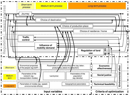
Fig. 1. Control model for the urban environment
Related to the possibly applicable measures and interventions influencing the operation efficiency of the urban environment, it has to be emphasized that the validity period of the decisions determines the complexity of the problem. For example, as it was examined the effects of a measure that is valid in short-term we can be assumed for the solution of the medium-term and the long-term decision problems to be fix parameters since e.g. an interim road maintenance work probably does not influence the choice of residence and production place.
However it has to be emphasized that according to the theory of “organic-urban environment” urban-planning should not focus on the solution of particular technological problems but on connecting segregated social groups and making urban-environment liveable (Jávor 2005). Hence every decision support system related to the urban environment should only be applied as an orientation tool for stakeholders.
The basic model
The applied basic model was developed by the authors; however it does not introduce any scientific innovation in the field of spatial general equilibrium models.
The urban environment is spatially divided into locations. These locations are linked with each other. Let us assume that each link aggregates all the possible routes between two locations (e.g. average distance). There is “i” amount of locations (zones) in the model. There are producers in every zone and all producers are specialized, hence there are “i” types of product. In case of special modelling it could be important to extend the model to order more producers to certain zones (see Anas et al., 2007). Firm makes no profit at any scale of operation (zero profit condition). “j” types of consumers are considered in the model to be able to describe different consumer groups.
There are different types of consumers in every zone and all types of consumers supply labour for one type of producers. Consumers travel from home to work and from home go shopping, generating income (1) and buying their demanded quantities of each differentiated good at each location. This pattern of shopping occurs because the consumer considers goods purchased from each location as essential commodity (this means also that each consumer will want to visit each). Land is involved in this simple model however it can be easily extended (see Anas et al., 2007). Furthermore it is necessary to be mentioned, that there is only one producer in the same location, but products are able to be substituted according to the Cobb-Douglas type utility (7) function hence pricing of commodities are quasi-competitive and vary among locations at equilibrium. The consumers take their location of employment and the shopping locations as given. Consumers are price takers in all markets and take as given all transport costs and travel times. The consumer chooses home locations and the shopping trip pattern. In the Cobb Douglas utility function, we assume that the taste coefficients a11..aij are different across consumers and that Σiaij=1 for every i product (homogeneity of degree one). Producers decide how much labour to demand. The equilibrium conditions involve product market and labour market (8). The equations presented below describing the defined model are derivable from the traditional consumer-producer constrained optimization problem (see Samuelson et al).
| Lj * (Wj – Tij) – Pi * ΣiXij = 0 | (1) |
| (Pk + Tkl) * Xkl / ckl – (Pi + Tij) * Xij / cij = 0 | (2) |
| Lj – Lsum * Uj / ΣiUj = 0 | (3) |
| Wi – Pi * aij * ΣjXij / Li = 0 | (4) |
| Pi – (Wiawi) / awiawi = 0 | (5) |
| ΣjXij – Li awi = 0 | (6) |
| Uj – πiXijcij = 0 | (7) |
| Lsum – ΣjLj = 0 | (8) |
Where:
Uj: utility of consumers living in zone j (variable),
Xij: consumption of inhabitants living in zone j, visiting zone i hence choosing product or service type i (variable),
cij: Cobb-Douglas taste coefficients of product or service type i consumed in zone j
(variable),
| awj: | Cobb-Douglas production parameter of labour used in zone j (parameter), |
| Lj: | consumer living in zone j (variable), |
| Pi: | price in zone i (variable), |
| Wi: | wage in zone i (variable), |
| Lsum: | the amount of labour available in the urban area (parameter), |
| Tij: | transport cost (parameter). |
Defining the optimal measure toolkit of urban development
The below presented methodology was developed by the authors. With this new approach, it is possible to define optimal measure toolkit, which maximizes the positive effect of transport interventions on social welfare.
The optimal measure toolkit of urban development should lead to the maximum or minimum value of one or more system components’ objective function. As it was mentioned above, the model contains two basic system components: consumers and producers. Since the developed control model is mostly focused on interventions related to the transport network, hence transport cost seems to be the adequate attribute to describe the effect of urban development measures. Accordingly, if we assume transport cost to be a system variable, we need to define i * j additional equations to keep the equation system solvable.
With the introduction of an additional constrained optimization problem the extended equation system can remain solvable. Since the aim of the extension is to define optimal public decisions (e.g. transport network development), it seems to be obvious that the chosen interventions should increase the objective function of a system component (consumers, producers). On the one hand consumers seem to be the better choice, because society consists of the individuals – and public decisions should primary support society. However, on the other hand deducing the form of social welfare function (corresponding to individual utility function) cannot be the scientific task of the economist according to Samuelson. Taking into account Samuelson’s consideration, social welfare function can be carefully applied by paying attention to only being interpreted in a relative term (for comparison), which still satisfies our objectives.
First the commodities demanded by consumers have to be derived from equation (2) so that consumption is dependent on transport cost.
Xij – cij * (Lj * (Wj – Tij)) / (Pk + Tkl) = 0 (9)
This equation contains one or two variables depending on whether Tij = Tkl or not. If they are equal it means that individuals in the Lj consumer group go shopping to the same location as working.
Figure 2. presents the effect of transport cost on consumption, where Tij is the cost of transport to work, Tkl is the cost of transport to the place of consumption and Xij is the amount of consumed goods.
It can be observed that an increase in both the costs of travel to shopping and working induce a decrease of consumption. This phenomenon suits the behaviour of rational consumer, since if travel costs to work increase, then consumers’ income will reduce. The same result can be observed in case of travel to the place of consumption getting more
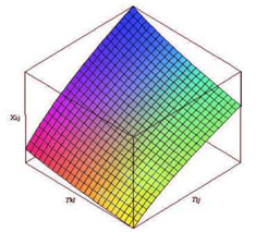
Fig. 2. The effect of transport on consumption
expensive, because then consumers can buy less commodity with the same income. Applying the new equations the social welfare function can be defined, which now can be the objective function of the constrained optimization problem.
Uj – πi (cij * (Lj * (Wj – Tij)) / (Pk + Tkl))cij = 0 (10)
The objective function will be constrained by the available development budget due to the limited nature of public resources. To be able to derive the solution of the maximization problem, constraint has to contain the variables of the objective function, so the constraint has to be based on transport cost. The equation below represents a possible way of formulating the constraint condition of public decision.
D – (Tij –Nij) * UN = 0 (11)
Where:
D: available public resources (parameter),
Tij: cost of travel to consumption place between zone i and j after development (variable),
Nij: cost of travel to consumption place between zone i and j before development
(variable),
UN: cost of a unit of transport development (parameter),
Now the Lagrangian can be derived from equation (11), (12) of constrained maximization problem.
Lagrangian1 = πj Uj(Tij)-λ * (D – (Tij –Nij) * UN) = 0 (12)
The equation (12) presents the relation between transport cost from home to work and to the shops. The equation has to be derived for three cases. If the place of work and consumption are different there are two derived variables in the equation, and if the consumer works and consumes in the same zone there is only one variable in the equation. The above presented method is applicable to involve transport network in general equilibrium models as an internal variable, which allow us to define optimal development interventions maximizing social welfare function.
Optimal measure toolkit of urban development – Numerical method
In the previous section transport cost was involved in the general equilibrium model as a continuous, internal variable. An example is presented below (provided by the authors), although practical application of the methodology will in the next step of the research be demonstrated.
To present a simple example, which can fit to the above mentioned conditions, we applied the equation system of the basic model but extended it with a transport development module. The parameters of the basic model were set to queasy-symmetric. So every cij = 0.33, , awj = 0.5, Lsum = 10. The only asymmetric part of the model is the arbitrarily chosen relation matrix below, which defines the home-work pairs. The definition of the matrix was led by the objective of ensuring that only differing locations are ordered together as a home – work pair.
Location of home
1 2 3
 | 1010 2 0013100 |
Table 1. Relation matrix of home – work location pairs
Finally the equation system has to be solved. Change in Tij represents the result of public resource allocation. To be able to evaluate the results the equation system is solved for four basic cases, which can provide us points of reference. First the equation system is solved with a basic transport network (no intrazonal travel time representation), the transport cost matrix of which is presented below.
Location of home
1 2 3
 | 110-72*10-22*10-2 2 2*10-210-7 32*10-22*10-210-7 |
Table 2. Basic transport cost matrix
Table 3. contains the results of the different solutions. There are twenty variables and five cases. The variables have already been introduced related to the basic model. The “A” case represents the “do nothing” case. The “B” case represents the effect of a transport cost reducing intervention between location 1 and to 2. In case “C” all transport costs have been reduced symmetrically. In case “D” the same transport cost reducing measure was concentrated on two links asymmetrically. The “E” case represents the optimal solution of resource allocation based on the conditions of the constraint function. Where the cost of a unit of transport development is one (UN=1) and available public resources are 0.0009 (D=0.0009).
| Variable | A | B | C | D | E |
| L1 | 3,33331 | 3,33334 | 3,33332 | 3,32991 | 3,333333 |
| L2 | 3,33332 | 3,33167 | 3,33332 | 3,33505 | 3,333333 |
| L3 | 3,33332 | 3,33499 | 3,33332 | 3,33501 | 3,333333 |
| X11 | 1,12615 | 1,11211 | 1,12386 | 1,12382 | 1,111873 |
| X12 | 1,10352 | 1,10967 | 1,10468 | 1,10273 | 1,11073 |
| X13 | 1,10352 | 1,11159 | 1,10468 | 1,10343 | 1,11073 |
| X21 | 1,10352 | 1,10971 | 1,10468 | 1,10247 | 1,11073 |
| X22 | 1,12671 | 1,11173 | 1,12427 | 1,12704 | 1,111874 |
| X23 | 1,10298 | 1,11030 | 1,10429 | 1,10529 | 1,110729 |
| X31 | 1,10352 | 1,11150 | 1,10468 | 1,10327 | 1,11073 |
| X32 | 1,10298 | 1,11017 | 1,10429 | 1,10533 | 1,110729 |
| X33 | 1,12671 | 1,11321 | 1,12427 | 1,12625 | 1,111874 |
| P1 | 1,00000 | 1,00010 | 1,00000 | 1,00061 | 1 |
| P2 | 1,00000 | 1,00024 | 1,00000 | 0,99954 | 1 |
| P3 | 1,00000 | 0,99966 | 1,00000 | 0,99984 | 1 |
| W1 | 1,03046 | 1,00275 | 1,02590 | 1,03015 | 1,001571 |
| W2 | 1,03046 | 1,00305 | 1,02590 | 1,02802 | 1,001571 |
| W3 | 1,03046 | 1,00184 | 1,02590 | 1,02864 | 1,001571 |
| Lsum | 9,99997 | 10,00000 | 9,99998 | 9,99998 | 10 |
Usum 3,32953 3,32956 3,32961 3,32956 3,329751
Table 3. Results
Summing up the results, it is clear that the change in transport costs indirectly affect customers’ utility. Investigating case “B” we can see that the asymmetric intervention (Tij between location 1 and 2 became 1,8*10-2) enhanced social welfare, however a sensible shift in the equilibrium can be observed.
In case “C” the interventions were symmetric (Tij between all locations were reduced to 1,8*10-2). It was expectable, that this more intensive “measure toolkit” enhanced social welfare function more and of course equilibrium remained symmetric.
In case “D” the interventions were asymmetric again. The total transport cost decline were the same as in case “C”, however transport cost of link between location 1 and 2 was reduced with one unit, transport cost of link between location 2 and 3 was reduced with two units and transport cost of link between location 3 and 1 was reduced with three units. In this case the social welfare grew less than in the symmetric case.
In case “E” the optimal solution was defined. The optimal solution was symmetric and compared to other alternatives optimal solution generated the maximum value of social welfare function, how it expectable was.
Conclusion
In earlier times – as we have seen – travel time, speed and capacity problems already made people try to estimate mobility demand. OD matrices describing mobility demand between zones are traditionally assumed to be constant. However, when a network operates close to its capacity, then a realistic traffic assignment would modify the network’s travel time matrix. That engenders changes in residence and production-place-choices and in long term this phenomenon would affect mobility demand structure and so the origin-destination matrix as well. Hence the assumption of constant demand does not prove to be realistic.
The continuous development of SCGE (spatial computable general equilibrium) models has made it possible to describe the behaviour of actors playing various roles in geographically closed economic space. Nowadays SCGE models can be applied at acceptable estimation efficiency to evaluate the expected spatial economic structure and the development of a given region.
Beside the traditionally produced output variables of general equilibrium models (e.g.: process, wages, rents) transportation cost or travel time can be involved in the equation system so as to be able to define the optimal measure toolkit leading to more efficient transport network . This approach makes it possible to enhance the efficiency of urban development processes, and beside this, it extends the traditional engineering approach by involving demand matrices in modelling process endogenously.
Thus a new module of equilibrium models has been introduced, which makes it possible to support the transport development. In this way it is possible to optimise our interventions on the investigated system.
In conclusion, the efficiency of urban transportation is getting more and more important because of the increase rate of mobility demand. To plan, control and organize urban transportation in the most efficient way, we also need to consider the aspects of land use. To handle both of the above mentioned urban planning areas, we shall develop models able to pay attention to all of their restrictive factors within temporal properties.