
Introduction
The previous model determined the number of trips produced by and attracted to each zone within the study area under scrutiny. For the trips produced by the zone in question, the trip distribution model determines the individual zones where each of these will end. For the trips ending within the zone under examination, the individual zone within which each trip originated is determined. The model thus predicts zone-to-zone trip interchanges. The process connects two known sets of trip ends but does not specify the precise route of the trip or the mode of travel used. These are determined in the two last phases of the modelling process. The end product of this phase is the formation of a trip matrix
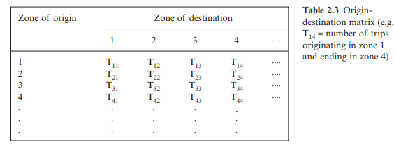
between origins and destinations, termed an origin-destination matrix. Its layout is illustrated in Table 2.3. There are several types of trip distribution models, including the gravity model and the Furness method.
The gravity model
The gravity model is the most popular of all the trip distribution models. It allows the effect of differing physical planning strategies, travel costs and transportation systems to be taken into account. Within it, existing data is analysed in order to obtain a relationship between trip volumes and the generation and attraction of trips along with impedance factors such as the cost of travel.
The name is derived from its similarity to the law of gravitation put forward by Newton where trip interchange between zones is directly proportional to the attractiveness of the zones to trips, and inversely proportional to some function of the spatial separation of the zones.
The gravity model exists in two forms:
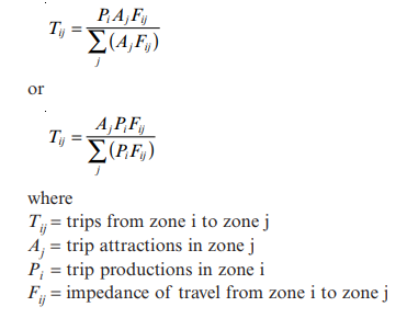
The impedance term, also called the deterrence function, refers to the resistance associated with the travel between zone i and zone j and is generally taken as a function of the cost of travel, travel time or travel distance between the two zones in question. One form of the deterrence function is

The impedance function is thus expressed in terms of a generalised cost function Cij and a term which is a model parameter established either by analysing the frequency of trips of different journey lengths or, less often, by calibration.
Calibration is an iterative process within which initial values for Equation 2.4 are assumed and Equation 2.2 or 2.3 is then calculated for known productions, attractions and impedances computed for the baseline year. The parameters within Equation 2.4 are then adjusted until a sufficient level of convergence is achieved.
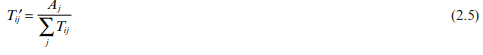
As illustrated by Equations 2.2 and 2.3, the gravity model can be used to distribute either the productions from zone i or the attractions to zone j. If the calculation shown in Example 2.1 is carried out for the other five zones so that T2j , T3j , T4j , T5j and T6j are calculated, a trip matrix will be generated with the rows of the resulting interchange matrix always summing to the number of trips produced within each zone because of the form of Equation 2.2. However, the columns when summed will not give the correct number of trips attracted to each zone. If, on the other hand, Equation 2.3 is used, the columns will sum correctly whereas the rows will not. In order to generate a matrix where row and column values sum correctly, regardless of which model is used, an iterative correction procedure, termed the row–column factor technique, can be used. This technique is demonstrated in the final worked example in section 2. It is explained briefly here.
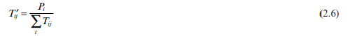
Assuming Equation 2.2 is used, the rows will sum correctly but the columns will not. The first iteration of the corrective procedure involves each value of Tij being modified so that each column will sum to the correct total of attractions.
Following this initial procedure, the rows will no longer sum correctly. Therefore, the next iteration involves a modification to each row so that they sum to the correct total of trip productions.
This sequence of corrections is repeated until successive iterations result in changes to values within the trip interchange matrix less than a specified percentage, signifying that sufficient convergence has been obtained. If Equation 2.3 is used, a similar corrective procedure is undertaken, but in this case the initial iteration involves correcting the production summations.


Comments are closed