The bridges, which link past to present and age gracefully, are one of the most important engineering structures. The bridges with different characteristics, thanks to their views, effects, and feelings during passing on, holds around and locations bring together the people for ages. In early applications, the bridges were designed as short span and narrow with stone and wood materials, and be able to carry light loads. But, nowadays, these conventional bridges have been replaced to steel and reinforced concrete.
There are various bridge types constructed during the last century according to the carrier system type, span lengths, and material properties such as masonry arch bridges, long span concrete/steel/composite highway bridges, base isolated bridges, footbridges, steel bridges, suspension bridges, cable-stayed bridges, and wooden/timber bridges. Masonry bridges have been built worldwide for social, economic, and strategic purposes. Originally intended to carry only pedestrian and horse-drawn vehicles, many of these historical bridges currently serve as critical components of transportation systems and, thus, must withstand significantly larger loads. Among various types of civil engineering structures, long span highway bridges, which are commonly used for passing large rivers, dam reservoirs, and deep valleys, attract the greatest interest for study particularly in terms of structural performance. Footbridges are generally situated to allow pedestrians to cross water or railways in areas where there are no nearby roads to necessitate a road bridge, and also across busy roads to let pedestrians cross safely without slowing down the traffic. Steel offers many advantages to the bridge builder, not only the material itself, but also its broad architectural possibilities such as high strength-to-weight ratio, high-quality material, speed of construction, versatility, modifications, recycling, durability, and aesthetics. Suspension and cable-stayed bridges are widely used across long spans (>550 m) and give rise to the usage of domains under the bridge. For this reason, the uses of suspension and cable-stayed bridges have increased recently. Wood is one of the most used and common materials for bridge constructions from the ancient times when humans first started finding ways on how to cross rivers and hard terrains.
Determination of dynamic response of bridges under static and dynamic loads, such as wind, earthquake, or traffic, is very complex and requires special studies. Finite element method has been widely used in civil engineering application since 1950s. Static, dynamic, linear, and nonlinear behavior can be obtained and illustrated using this method. It is generally expected that finite element models (FEMs) based on technical design data and engineering judgments can yield reliable simulation. However, because of modeling uncertainties, these models often cannot predict dynamic characteristics with the required level of accuracy. This raises the need for verification of finite element models using nondestructive experimental measurement tests.
There are two basically different methods available to experimentally identify the dynamic system parameters of a structure: experimental modal analysis (EMA) and operational modal analysis (OMA). In the EMA, the structure is excited by known input forces and the structural behavior is evaluated. In the OMA, the ambient vibrations such as vehicle load, wind, or wave loads have been used to actuate the structures. Heavy forced excitations may become expensive and sometimes may cause damage to the structure. Ambient excitations and their combination are environmental or natural excitations. Structural identification using this method gains the major importance. In this case, only response data of ambient vibrations are measurable while actual loading conditions are unknown. A system identification procedure will therefore need to base itself on output-only data.
It is well accepted that the finite element model updating is used to minimize the differences between analytically and experimentally determined dynamic characteristics by changing some uncertain parameters such as material properties, boundary conditions, section and connection details, and some additional structural elements and weights. In the finite element model updating, determination of the uncertain parameters and their ratios/values can be decided according to the nondestructive testing methods such as visual inspection, half-cell electrical potential method, Schmidt rebound hammer test, carbonation depth measurement test, permeability test, penetration resistance or Windsor probe test, resistivity measurement, electromagnetic methods, radiographic testing, ultrasonic testing, infrared thermography, ground penetrating radar, radioisotope gauges, acoustics emission, computed tomography, strain sensing, and corrosion rate measurement. The detailed information can be found in the related literature.
Modal parameter estimation methods
ENHANCED FREQUENCY DOMAIN DECOMPOSITION (EFDD) METHOD
Enhanced frequency domain decomposition (EFDD) method is an extension of frequency domain decomposition (FDD) method which is a basic and easy-to-use method. In this method, modes are simply picked locating the peaks in singular value decomposition plots [1, 2].
In EFDD, the single degree of freedom (SDOF) power spectral density (PSD) function, identified around a peak of resonance, is taken back to the time domain using the Inverse Discrete Fourier Transform. In EFDD method, the relationship between unknown input and measured responses can be expressed as :

where Gxx{jw} is the PSD matrix of the input, Gyy{jw} is the PSD matrix of the responses, H{jw} is the frequency response function (FRF) matrix, and * and superscript T denote complex conjugate and transpose, respectively. The FRF can be written in partial fraction, i.e., pole/residue form as [4]

where n is the number of modes, λk is the pole, and, Rk is the residue. Substituting Eq. (2) into (1), we have

where s is the singular value, superscript H denotes complex conjugate and transpose. Multiplying the two partial fraction factors and making use of the Heaviside partial fraction theorem, the output PSD can be reduced to a pole/residue form as follows:

where Ak is the kth residue matrix of the output PSD. In the EFDD identification, the first step is to estimate the PSD matrix. The estimation of the output PSD, Gyy(jw) known at discrete frequencies w = wi is then decomposed by taking the SVD of the matrix

where the matrix Ui=[ui1,ui2,….,uim] is a unitary matrix holding the singular vectors, uij, and Si is a diagonal matrix holding the scalar singular values sij [4–6].
STOCHASTIC SUBSPACE IDENTIFICATION (SSI) METHOD
Stochastic subspace identification (SSI) method is an output-only time domain method that directly works with time data, without the need to convert them to correlations. The model of structural vibrations can be defined by a set of linear, constant coefficient and second-order differential equations [7]:

where M, C2, and K are the mass, damping, and stiffness matrices, F(t) is the excitation force, and U(t) is the displacement vector depending on time t. Note that the force vector F(t) is factorized into a matrix B2 describing the inputs in space and a vector u(t). The equation of dynamic equilibrium (6) will be converted to a more suitable form: the discrete-time stochastic state-space model [7, 8]. With the following definitions

Eq. (6) can be transformed into the state equation

where A is the state matrix, B is the input matrix, and x(t) is the state vector. If it is assumed that the measurements are evaluated at only one sensor location, and that this sensor can be accelerometer, velocity, or displacement transducer, the observation equation is [9]:
![]() where C is the output matrix and D is the direct transmission matrix. Eqs. (8) and (9) constitute a continuous-time deterministic state-space model. This is not realistic: measurements are available at discrete time instants kΔt, k ∈ N with Δt, the sample time and noise is always influencing the data. After sampling, the state-space model looks like [6]:
where C is the output matrix and D is the direct transmission matrix. Eqs. (8) and (9) constitute a continuous-time deterministic state-space model. This is not realistic: measurements are available at discrete time instants kΔt, k ∈ N with Δt, the sample time and noise is always influencing the data. After sampling, the state-space model looks like [6]:
![]() where xk = x(kΔt) is the discrete-time state vector. The stochastic components are included and obtained discrete-time combined deterministic-stochastic state-space model:
where xk = x(kΔt) is the discrete-time state vector. The stochastic components are included and obtained discrete-time combined deterministic-stochastic state-space model:
![]() where wk is the process noise due to disturbances and modeling inaccuracies and vk is the measurement noise due to the sensor inaccuracy. They are both immeasurable vector signals but we assume that they are zero mean, white, and covariance matrices [7]:
where wk is the process noise due to disturbances and modeling inaccuracies and vk is the measurement noise due to the sensor inaccuracy. They are both immeasurable vector signals but we assume that they are zero mean, white, and covariance matrices [7]:
![]() where E is the expected value operator and δpq is the Kronecker delta. This is a function of two variables, usually integers, which is 1 if they are equal, and 0 otherwise. It can be written as the symbol δpq, and treated as a notational shorthand rather than a function:
where E is the expected value operator and δpq is the Kronecker delta. This is a function of two variables, usually integers, which is 1 if they are equal, and 0 otherwise. It can be written as the symbol δpq, and treated as a notational shorthand rather than a function:

The vibration information that is available in structural health monitoring is usually the responses of a structure excited by the operational inputs that are some immeasurable inputs. It is impossible to distinguish deterministic input uk from the noise terms wk, vk in Eq. (11). If the deterministic input term uk is modeled by the noise terms wk, vk the discrete-time purely stochastic state-space model is obtained:

Eq. (14) constitutes the basis for the time-domain system identification through operational vibration measurements.
MODAL ASSURANCE CRITERION
The modal assurance criterion (MAC) is defined as a scalar constant relating the degree of consistency (linearity) between one modal and another reference modal vector [10] as follows:
 where {∅ai}{∅ai} and {∅ej}{∅ej} are the modal vectors of ith and jth for different methods, respectively.
Nondestructive testing of bridges
In the content of this chapter, 10 different bridges that have different type and carrier systems are selected as case studies:
· Historical masonry arch bridges (Osmanlı, Mikron, and Şenyuva)
· Long span concrete highway bridges (Kömürhan and Birecik)
· Base isolated bridge (Gülburnu)
· Footbridges (Ortahisar and Akçaabat)
· Steel bridges (Eynel)
· Old riveted bridges (Borçka)
HISTORICAL MASONRY ARCH BRIDGES
Historical structures are identity of the communities. They are not only structures, which contain stone, timber, mortar, etc., they also contain the social culture and this is the biggest difference between the new structures. Almost every person is curious about the past and they want to learn some information of their ancestors. So the easiest way to learn about the past is to examine the historical data and structures. In the last century, people have given more attention to preserve the historical structures. A lot of studies have been carried out for estimating behavior of these structures and reliable restoration could be made to preserve them for future.
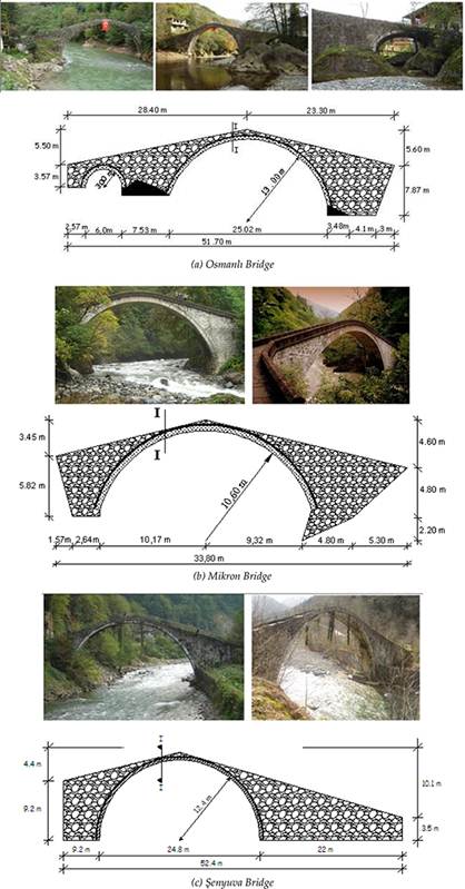
FIGURE 1.
Views of the historical masonry arch bridges with relieve drawings. (a) Osmanlı Bridge, (b) Mikron Bridge, and (c) Şenyuva Bridge.
Masonry arch bridges hold an important place in historical structures [11]. They are not complex structures. A stone arch bridge consists of stone blocks and mortar joints. Blocks have high strength in compression and low strength in tension while mortar has generally low strength. Historical masonry arch bridges are vital components of transportation systems in many countries worldwide, ensuring the ready access of goods and services to millions of people [12]. Many of those bridges, which were originally built for the passage of carts, are being used for road and rail vehicles. They demonstrate a surprisingly high load bearing capacity and good durability.
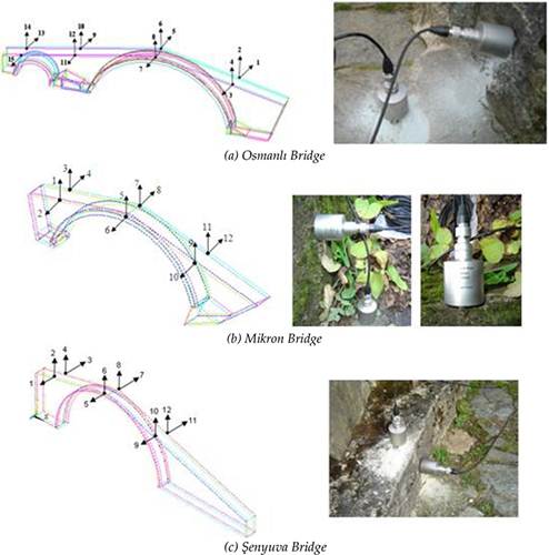
FIGURE 2.
Accelerometer locations and views from the measurements. (a) Osmanlı Bridge, (b) Mikron Bridge, and (c) Şenyuva Bridge.
Osmanlı, Mikron, and Şenyuva historical masonry arch bridges constructed in Turkey are selected for example. The Osmanlı historical masonry arch bridge was built in the nineteenth century. This two-spanned arch bridge has a total length of 51.7 m. The span of each arch is 25.2 and 6 m, and the radius of each arch is 13 and 3m, respectively.
The Mikron historic arch bridge, built in the mid-nineteenth century during the Ottoman Empire, spans the Fırtına River in Rize, Turkey. Cut stone blocks composed the bridge’s arches and parapets. In 1998, Turkey’s General Directorate for Highways supervised repair of the main structural elements of the bridge (stone arches, side walls, and filler material). The bridge, with a total length of 33.80 m, has two stone, inner and outer semi-circular arches, which have thicknesses of 0.50 and 0.15 m, respectively.
The Şenyuva historical arch bridge built in 1696 by the native population is located on Fırtına Stream in Çamlihemşin, Rize, Turkey. The bridge has a single arch. The total span of bridge is 52.4 m, the span of the bridge arch is 24.8 m, the height of the arch is 12.4 m, and the wide of the deck is 2.5 m. Height of the side walls at both side are 9.2 and 3.5 m, respectively. There are 60 cm × 30 cm dimensional parapets on both sides of the bridge deck. Some views of the bridges with relieve drawings are given in Figure 1(a–c).
Ambient vibration tests were performed under existing environmental condition. B&K 8340 and B&K 3560 experimental measurement equipment were used. PULSE [13] and OMA [14] softwares were used to signal processing and parameter estimations. Accelerometer locations and views from the measurements for each bridge are shown in Figure 2.
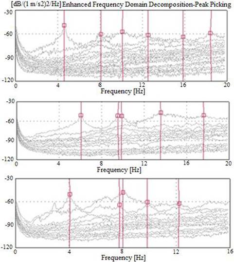
FIGURE 3.
The singular values of spectral density matrices for historical masonry arch bridges.
Accelerometer setups shown in Figure 2 were used, and measurements were carried out for at least 30 min. The singular values of spectral density matrices are given in Figure 3. The dynamic characteristics are given in Table 1 and Figure 4. The first four natural frequencies are obtained between 4 and 14 Hz. The mode shapes occurred as lateral and vertical forms.
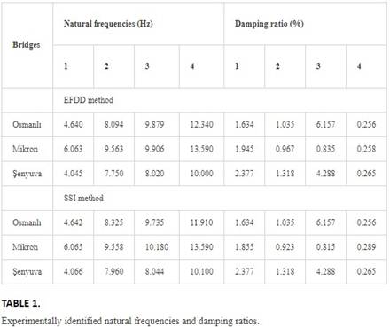
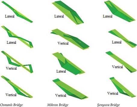
FIGURE 4.
The first four mode shapes of the historical masonry arch bridges.
LONG SPAN CONCRETE HIGHWAY BRIDGES
Kömürhan and Birecik long span concrete highway bridges constructed in Turkey are selected for example. The bridge deck consists of a main span of 135 m and two side span of 76 m each. The total bridge length is 287 m and width of the bridge is 11.50 m. The structural system of Kömürhan Highway Bridge consists of deck, columns, side support, and expansion joint. The deck of the bridge was constructed with balanced cantilever and prestressed box beam method. There are two main columns of 59.50 m each. Foundation of the main column is concrete in mass having the dimension of 24 m × 13.5 m and 5 m depth. To combine deck cantilevers, an expansion joint is constituted in the main span of the bridge [16, 17].
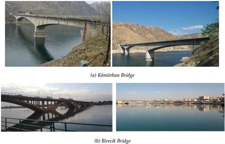
FIGURE 5.
Some views of the long span concrete highway bridges with relieve drawings. (a) Kömürhan Bridge and
(b) Birecik Bridge.
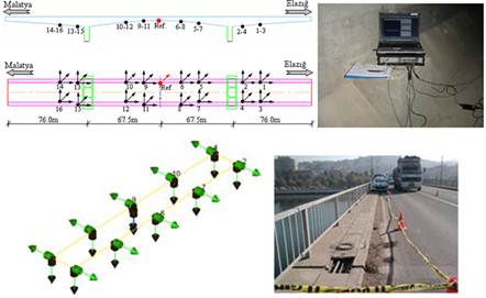
FIGURE 6.
Accelerometer location and views from the measurements.
Birecik Bridge is located 81 km of the Şanlıurfa-Gaziantep state highway over Fırat River in Turkey. The construction of the bridge was started in June 1951 and the bridge was opened to the traffic in April 1956. The bridge consist of five arches, each arch has a 55 m main span. The total bridge length is 300 m and the width of the bridge is 10 m. The bridge arches have rigid connectivity at middle spans and side supports. But, right and left side of the middle points of slabs are constructed using joints. Columns, beams, arches, decks, and foundations were constructed as reinforced concrete [18]. Some views of the bridges with relieve drawings is given in Figure 5. Figure 6 presents the accelerometer location and views from the measurement. The measurements were carried out for at least 60 min. The singular values of spectral density matrices obtained from vibration data are given in Figure 7.
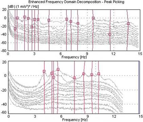
FIGURE 7.
The singular values of spectral density matrices for long span highway bridges.
The dynamic characteristics and related mode shapes are given in Table 2 and Figure 8. The first four natural frequencies are obtained between 0.7 and 2.3 Hz for the Kömürhan Bridge and 2.4 and 4.6 Hz for the Birecik Bridge, respectively. The mode shapes occurred in lateral, vertical, and torsional forms.
| Bridges | EFDD method | |||||||
| Natural frequencies (Hz) | Damping ratio (%) | |||||||
| 1 | 2 | 3 | 4 | 1 | 2 | 3 | 4 | |
| Kömürhan | 0.788 | 1.027 | 1.850 | 2.291 | 1.373 | 1.785 | 2.057 | 1.465 |
| Birecik | 2.496 | 3.115 | 3.378 | 4.545 | 4.358 | 0.899 | 0.863 | 0.118 |
TABLE 2.
Experimentally identified natural frequencies and damping ratios.
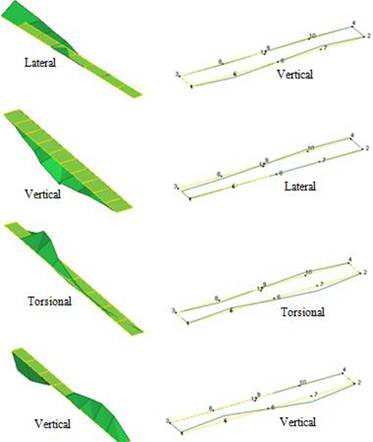
FIGURE 8.
The first four mode shapes of the long span highway bridges.
BASE ISOLATED BRIDGE
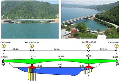
FIGURE 9.
Some views of the base isolated bridge with relieve drawings.
Base isolated Gülburnu Highway Bridge constructed in Turkey is selected for example. The construction of the bridge was started in November 2005 and the bridge was opened to the traffic in May 2009. The bridge is twin prestressed concrete box girder structures. The bridge deck consists of a main span of 165 m and two side span of 82.5 m each. The total bridge length is 330 m and the width of the bridge is 30 m. The structural system of the bridge consists of deck, piers, and side support. There are four piers and each has 4.50 m height and 9.00 m × 3.75 m cross-section areas. All piers are footed on the two raft foundation with bored piles. Two abutments that allow longitudinal direction movement only support the superstructure at both sides [19, 20]. Some views of the bridge with relieve drawings is given in Figure 9.
Accelerometer locations are shown in Figure 10. The measurements were carried out for at least 60 min. The singular values of spectral density matrices obtained from the processing vibration data are given in Figure 11.
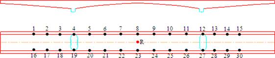
FIGURE 10.
Accelerometer location and views taken from the measurements.
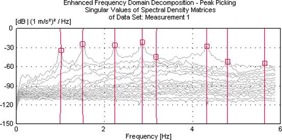
FIGURE 11.
The singular values of spectral density matrices for base isolated bridge.
| Mode | Natural frequencies (Hz) | Damping ratio (%) | ||
| EFDD | SSI | EFDD | SSI | |
| 1 | 0.993 | 0.995 | 2.661 | 3.952 |
| 2 | 1.508 | 1.505 | 0.958 | 0.559 |
| 3 | 2.238 | 2.241 | 0.741 | 0.604 |
| 4 | 2.853 | 2.874 | 0.765 | 2.145 |
| 5 | 3.181 | 3.258 | 0.371 | 0.758 |
| 6 | 4.321 | 4.298 | 0.558 | 0.962 |
TABLE 3.
Experimentally identified natural frequencies and damping ratios.
Natural frequencies, mode shapes, and damping ratios are given in Table 3 and Figure 12. The first six natural frequencies are obtained between 0.9 and 4.5 Hz. The mode shapes occurred in vertical, torsional, longitudinal, and lateral forms.
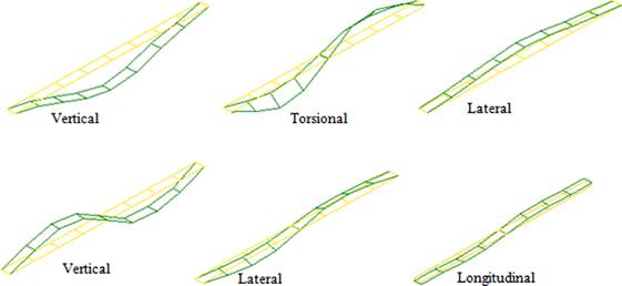
FIGURE 12.
The first six mode shapes of the base isolated bridge.
FOOTBRIDGES
Ortahisar and Akçaabat footbridges constructed in Turkey are selected for example. Ortahisar arch-type footbridge is located in a heavy traffic area in Trabzon, Turkey, and has a main span of 35 m. The footbridge operates as part of a pedestrian public footpath [21]. Akçaabat footbridge also operates as part of a pedestrian public footpath [22]. Some views of the footbridges with relieve drawings are given in Figure 13.
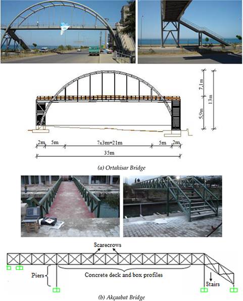
FIGURE 13.
Some views of the footbridges with relieve drawings. (a) Ortahisar Bridge and (b) Akçaabat Bridge.
Some views from the measurements with accelerometer locations are shown in Figure 14. The measurements were carried out for at least 45 min. The singular values of spectral density matrices obtained from the processing vibration data are given in Figure 15.
The dynamic characteristics such as natural frequencies, mode shapes, and damping ratios obtained using EFDD and SSI methods in frequency and time domain are given in Table 4 and Figure 16. The first six natural frequencies are obtained between 1.9 and 6.7 Hz. The mode shapes occurred in lateral and torsional forms.
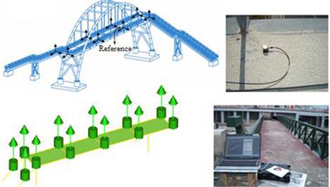
FIGURE 14.
Accelerometer location and views taken from the measurements.
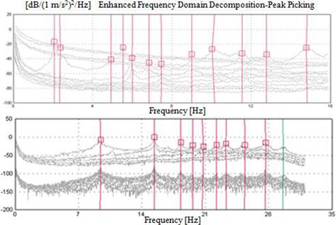
FIGURE 15.
The singular values of spectral density matrices for footbridges.
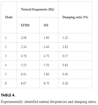
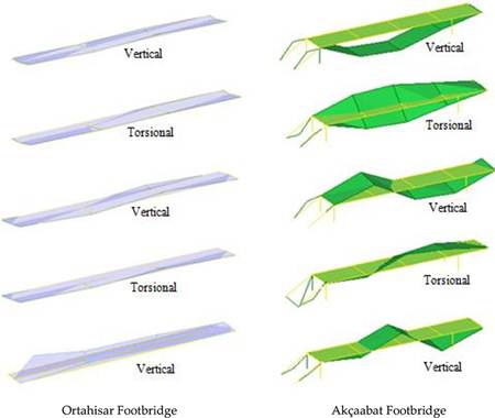
FIGURE 16.
The first five mode shapes of the footbridges.
STEEL BRIDGES
Bridges are one of the most important engineering structures which are commonly used for interplant and intercity transportation. In Turkey, in earlier days they were designed as narrow and short span with stone and wood materials and to be able to carry light loads. Today, the location of these bridges has been replaced with long span reinforced concrete and steel bridges. According to the General Directorate of Highways data, there are 6447 highway bridges with a total length of 296 km in Turkey.
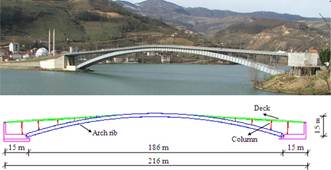
FIGURE 17.
Some views of the steel bridge with relieve drawings.
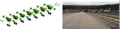
FIGURE 18.
Accelerometer location and views taken from the measurements.
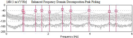
FIGURE 19.
The singular values of spectral density matrices for steel bridge.
Eynel steel bridge constructed in Turkey is selected for example. The bridge is located in the Black Sea region of Turkey. It connects to the villages near the two sides of Suat Uğurlu Dam reservoir in the city of Samsun. The construction of the bridge started in 2007 and it was opened to traffic in 2009. The bridge is upper-deck steel bridge which has arch-type carriage system with a total length of 216 m. The span of the arch rib is 186 m and it has box-type section. The height and width of the section is 2.4 and 12 m. The deck is 12 m wide and has a constant thickness of 10 cm [23]. Some views of the steel bridge are given in Figure 17.
In Figure 18, the accelerometer locations and views during the measurement are presented in detail. The measurements were carried out for at least 60 min. The singular values of spectral density matrices obtained from the processing vibration data are given in Figure 19.
Table 5 and Figure 20 summarize the dynamic characteristics obtained using EFDD and SSI methods. The first six natural frequencies are obtained between 0.7 and 2.7 Hz. The mode shapes occurred in lateral and transverse forms.
| Mode | Natural frequencies (Hz) | Damping ratio (%) | ||
| EFDD | SSI | EFDD | SSI | |
| 1 | 0.779 | 0.800 | 0.73 | 1.67 |
| 2 | 0.828 | – | 1.30 | – |
| 3 | 1.395 | 1.381 | 0.51 | 1.06 |
| 4 | 1.688 | 1.709 | 0.40 | 3.26 |
| 5 | 2.057 | 1.933 | 0.45 | 0.84 |
| 6 | 2.674 | 2.670 | 0.25 | 0.36 |
TABLE 5.
Experimentally identified natural frequencies and damping ratios.
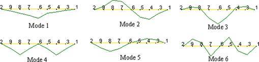
FIGURE 20.
The first six mode shapes of the steel bridge.
OLD RIVETED BRIDGE
Borçka Old Riveted Bridge constructed in Turkey is selected for example. The bridge, built in 1936, is on the Çoruh River in the town center of Borçka. Total length and width of the bridge are about 114 and 5.30 m, respectively. The main structural system of the bridge has an arch height of 16.30 m from the bridge deck. The bridge girders consist of two edge beams and five middle beams in the longitudinal and transverse directions. The structural elements (arches, pillars, decks, wind connections, etc.) are made out of steel with riveted connections. Bridge is closed to vehicle traffic and it is for only pedestrians [24]. Some views of the old riveted bridge with relieve drawings are given in Figure 21.
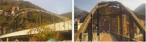
FIGURE 21.
Some views of the old riveted bridge with relieve drawings.
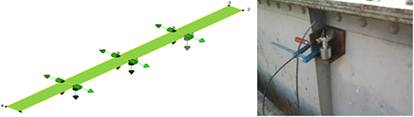
FIGURE 22.
Accelerometer location and views taken from the measurement.
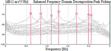
FIGURE 23.
The singular values of spectral density matrices for old riveted bridge.
| Mode | Natural frequencies (Hz) | Damping ratio (%) | ||
| EFDD | SSI | EFDD | SSI | |
| 1 | 0.970 | 0.968 | 2.185 | 1.801 |
| 2 | 1.352 | 1.348 | 0.736 | 0.926 |
| 3 | 1.761 | 1.758 | 0.962 | 0.817 |
| 4 | 2.042 | 2.041 | 0.459 | 0.401 |
| 5 | 2.726 | 2.725 | 0.764 | 0.707 |
| 6 | 3.183 | 3.189 | 0.432 | 0.395 |
TABLE 6.
Experimentally identified natural frequencies and damping ratios.
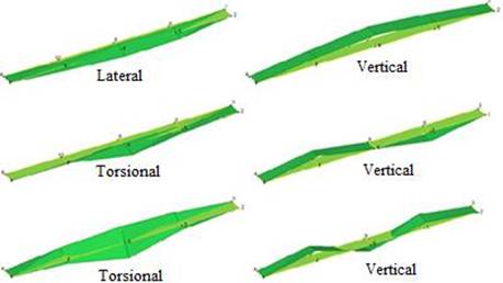
FIGURE 24.
The first six mode shapes of the old riveted bridge.
The accelerometer locations and placements on the deck are displayed in Figure 22. The measurements were carried out for at least 60 min. The singular values of spectral density matrices obtained from the vibration data are given in Figure 23.
The dynamic characteristics obtained using EFDD and SSI methods are given in Table 6 and Figure 24. The first six natural frequencies are obtained between 0.9 and 3.2 Hz. The mode shapes occurred in lateral, vertical, and torsional forms.
Finite element analyses and model updating
To validate the experimentally identified dynamic characteristics, finite element models of the bridges are constituted in the SAP2000 and ANSYS [25, 26] software. With modal analyses, the natural frequencies and related mode shapes are obtained (Figure 25). The analytically identified natural frequencies are summarized in Table 7.
It is seen that ambient vibration measurements are enough to identify the most significant modes of all bridge types. There is a good agreement between natural frequencies and corresponding mode shapes. The maximum differences are obtained as nearly as 10–20%. To eliminate these differences, the finite element models of the bridges should be updated by changing some uncertain parameters such as material properties, boundary conditions, section areas, etc. It can be evaluated that the maximum differences are reduced from 10–20 to 2–5% after model updating. More information can be found in the literature [11, 12, 15–18, 20–24, 27].
Also, to display the model updating effect, dynamic responses of the bridge are performed before and after model updating. It is seen that this procedure has vital importance to represent the real structural behavior. More information can be found in the literature [11, 12, 15–18, 20–24, 27].
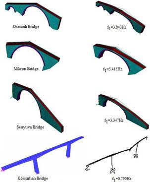
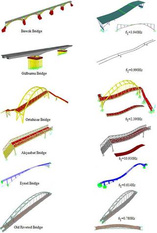
FIGURE 25.
The finite element models of the bridges with first mode shapes.
TABLE 7.
Natural frequencies identified by finite element analyses.
Conclusion
This chapter presents a comparative study about the nondestructive measurement of bridges for structural identification. Ten different bridges, which have different type and carrier systems, are selected as case studies. The dynamic characteristics such as natural frequencies, mode shapes, and damping ratios are extracted using ambient vibration tests with operational modal analysis procedure. The experimentally identified dynamic characteristics are validated by the finite element results, and the differences are evaluated.
It can be seen that the ambient vibration measurements are enough to identify the most significant modes of all bridge types.
The first natural frequencies are obtained as 4–14, 0.7–2.3, 2.4–4.6, 0.9–4.5, 1.9–6.7, 0.7–2.7, and 0.9–3.2 Hz for historical masonry arch bridges, Kömürhan and Birecik long span highway bridges, base isolated bridge, footbridges, steel bridges, and old riveted bridges, respectively.
The mode shapes occurred as vertical, lateral, longitudinal, and torsional forms. Especially, longitudinal modes should be considered for a base isolated bridge.
The finite element analyses are performed, and the results are compared with each other. It is seen that there is a good agreement between the natural frequencies and corresponding mode shapes. The maximum differences are nearly within 10–20%.
To eliminate these differences, the finite element models of the bridges should be updated by changing some uncertain parameters such as material properties, boundary conditions, section areas, etc. It can be evaluated that the maximum differences are reduced from 10–20 to 2–5% after model updating procedure. More information can be found in the cited articles.

