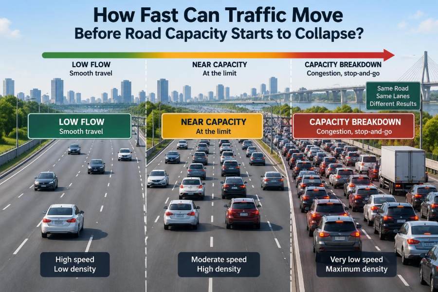

Picture a motorway that is moving freely at 100 km/h. A few minutes later, brake lights appear for no obvious reason. Vehicles slow, gaps disappear, and the queue begins to travel backward even though every driver is trying to move forward.
This experience creates a tempting conclusion: traffic would work better if everyone simply drove faster. Yet roads do not behave like empty runways. Their ability to carry vehicles depends on speed, spacing, lane changes, merging, vehicle mix, and how predictably people respond to one another.
For civil engineers, the central question is not just how fast vehicles can travel. It is how many vehicles can pass a point in a given time without the traffic stream becoming unstable.
That distinction shapes highway design, ramp control, signal timing, work-zone planning, speed management, and the daily trip of anyone using a busy road.
🚗 Speed Is Only One Part of Road Performance
A road’s performance is often described by three connected quantities: speed, flow, and density. Speed is how fast vehicles travel, flow is the number of vehicles passing a point per unit time, and density is the number of vehicles occupying a length of road.
Drivers notice speed first because it affects travel time. Engineers must also watch flow and density because a road can have high speeds while carrying relatively few vehicles.
An empty three-lane motorway may allow fast travel, but it is not carrying many people. A busy arterial may move slowly but still serve a substantial number of vehicles. The best operating condition depends on the road’s purpose, safety constraints, and demand.
📏 The Fundamental Traffic Relationship
The basic relationship is expressed as q = k × v, where q is flow, k is density, and v is average speed. Units must be consistent: for example, vehicles per hour equals vehicles per kilometre times kilometres per hour.
This simple equation is powerful because it explains why speed alone cannot represent capacity. At a given speed, adding vehicles raises flow only until the vehicles are close enough that their speed begins to fall substantially.
Traffic engineering commonly evaluates these measures by lane, because a three-lane road does not always operate like three identical independent lanes. Trucks, lane-changing, gradients, ramps, and uneven lane use can reduce the benefit of additional lanes.
⏱️ Headway Determines How Many Vehicles Fit
Time headway is the time between two successive vehicles passing the same point. If the average headway grows, fewer vehicles can pass in an hour. If it becomes very short, theoretical flow rises—but safety and stability become concerns.
At a steady 2-second headway, a lane could theoretically accommodate about 1,800 vehicles per hour. Real conditions vary because drivers do not maintain identical gaps, and large vehicles occupy more space and need longer braking distances.
Headway includes more than physical vehicle length. It reflects a driver’s perception, reaction, desired safety margin, vehicle performance, weather, and confidence in the surrounding traffic.
🛣️ Why Capacity Occurs Below Free-Flow Speed
On a lightly used freeway, vehicles can travel at their preferred or free-flow speed because they have ample space. Flow is low, however, because few vehicles are present.
As demand rises, more vehicles use the same road space. Flow increases even if average speed falls modestly. Eventually, the stream reaches a condition near capacity: the highest sustainable rate at which vehicles can pass a location under prevailing conditions.
Capacity therefore is not usually achieved at the highest possible speed. It occurs where vehicles are close enough to produce high flow but still have enough space to avoid frequent braking and disruptive interactions.
📈 Reading the Speed–Flow Curve
A speed–flow curve illustrates a common traffic pattern. At low flow, speed remains close to free-flow speed. As flow approaches capacity, speed becomes more sensitive to small disturbances.
Beyond the critical point, the flow may no longer be sustained. A brief brake application, an aggressive merge, or a lane change can trigger a queue. Vehicles then move slowly at high density, and the number passing the bottleneck may fall.
| Traffic condition | Typical speed pattern | Flow implication |
|---|---|---|
| Light traffic | Near free-flow speed | Low flow because few vehicles are present |
| Stable heavy traffic | Moderately reduced speed | High flow, often near practical capacity |
| Unstable near-capacity traffic | Variable speed and frequent braking | High but fragile flow |
| Congested traffic | Low, stop-and-go speed | Reduced discharge flow at the bottleneck |
The exact curve differs by facility and local conditions. It is a planning and analysis concept, not a promise that every roadway will behave identically.
⚠️ The Critical Point Is Fragile
Near capacity, drivers have little spare space or time to absorb changes. Traffic can appear acceptable one moment and deteriorate quickly the next.
This is why a road operating at 95% of its estimated capacity is not necessarily “fine.” The remaining margin may be too small to handle normal variation in arrivals, weather, driver behaviour, or a short-lived obstruction.
Engineers often seek reliable operation rather than pushing ordinary traffic right to the theoretical maximum. A slightly lower volume with steadier speeds can provide more predictable travel times.
🌊 How a Phantom Traffic Jam Forms
A phantom jam is a queue that appears without a crash, closed lane, or visible obstacle at its origin. It can begin when one driver brakes a little more sharply than necessary.
The following driver reacts later and brakes harder. Each reaction can amplify upstream until a dense wave forms. Drivers entering the wave slow down, while drivers leaving it accelerate, making the queue appear to move backward.
The road has not physically moved backward. The disturbance wave has. Near-capacity traffic is particularly vulnerable because the available gaps are too small to smooth out small speed changes.
🔄 Stop-and-Go Waves Reduce Useful Capacity
Stop-and-go traffic wastes road capacity because vehicles do not restart in a perfectly continuous stream. Drivers leave pauses, accelerate at different rates, and hesitate after braking.
At a bottleneck, the rate at which queued vehicles pass may be lower than the rate that was observed just before the breakdown. This effect is often called a capacity drop.
Its size varies by site and conditions, so it should not be treated as one universal value. The practical lesson is clear: preventing breakdown can be more effective than trying to recover after a long queue has formed.
🚦 Bottlenecks Set the Real Limit
A road corridor is constrained by its weakest operating point, not its widest or fastest segment. That limiting point may be a lane drop, a steep upgrade, a tunnel, a toll or control point, a busy interchange, or a signalized intersection.
When arrivals exceed what the bottleneck can discharge, a queue forms upstream. Adding capacity far upstream may only allow more vehicles to reach the queue faster unless the bottleneck itself is addressed.
Finding the true bottleneck requires observation and data. The longest queue is not always the location causing it; queues frequently extend far upstream from the source.
🔀 Merging Creates Turbulence
An on-ramp adds vehicles that must find acceptable gaps. Mainline drivers may change lanes or brake to create room, while entering drivers adjust their speed to fit the traffic stream.
These interactions create turbulence: speed variation and lane-changing that reduce the smoothness of traffic flow. A merge can operate well at moderate demand but become unstable when both the ramp and mainline are heavily loaded.
Good acceleration-lane design, clear markings, ramp metering where appropriate, and coordinated upstream operations can reduce this disturbance. None of these measures creates unlimited capacity; they help use the available capacity more consistently.
↔️ Weaving Is Harder Than a Simple Merge
Weaving occurs when vehicles entering a roadway need to cross paths with vehicles preparing to exit. A common example is the short section between a closely spaced entrance ramp and exit ramp.
Unlike a single merge, weaving requires movement across lanes in both directions. The issue is not merely the number of cars, but the number and urgency of lane-changing maneuvers.
Longer weaving lengths, collector-distributor roads, ramp spacing, and carefully selected interchange layouts can help. In constrained urban corridors, operational strategies may be needed because rebuilding the interchange can be costly and disruptive.
🚚 Heavy Vehicles Change the Traffic Stream
Trucks and buses are essential road users, but they do not affect capacity in the same way as passenger cars. They are longer, accelerate more slowly, need greater gaps, and can lose speed on grades.
Traffic analysis often accounts for this through passenger-car equivalents: a way to represent the additional operating effect of a heavy vehicle. The appropriate adjustment depends on terrain, lane configuration, and traffic conditions.
A small share of heavy vehicles may have little visible effect on a level freeway during off-peak periods. The same share can strongly affect a steep climbing section near capacity, especially when vehicles must change lanes to pass.
⛰️ Grades Can Turn a Fast Road Into a Queue Source
On an uphill grade, heavy vehicles may slow progressively. Faster vehicles then move into adjacent lanes, increasing lane-changing and creating uneven speeds across the carriageway.
If demand is already high, the slower-moving platoon can initiate breakdown. The issue is not that slower vehicles are inherently a problem; it is that a speed difference within dense traffic demands more passing and merging.
Climbing lanes, grade-aware design speeds, and freight-sensitive traffic analysis are common responses. Their value depends on the grade length, truck volumes, available right-of-way, and downstream constraints.
🌧️ Weather Shrinks the Operating Envelope
Rain, snow, fog, glare, and strong winds can reduce visibility, tire-road friction, and driver confidence. Sensible drivers compensate by increasing headway and reducing speed.
That choice may lower a lane’s practical capacity, but it can also reduce crash risk. Trying to preserve dry-weather throughput during poor conditions by encouraging high speed would ignore the physical reason drivers need more space.
Variable speed limits, clear warnings, drainage maintenance, pavement surface management, and incident response can support safer operations. The appropriate speed should reflect conditions, not only a posted number.
🧱 Work Zones Have More Than One Constraint
A work zone may reduce lanes, narrow lanes, shift alignments, lower speeds, and introduce construction vehicles. Each feature can affect flow, but the narrowest visible section is not always the only limitation.
Early braking at warning signs, late merges, uneven lane use, and unfamiliar geometry can generate queues before the actual lane closure. Work-zone planning should consider the full approach, taper, activity area, and recovery area.
Scheduling, temporary traffic control, clear advance information, and realistic queue-management plans matter. Worker safety remains the primary constraint; capacity is not a reason to compromise safe work-zone design.
🚥 Intersections Measure Capacity in Green Time
At a signalized intersection, capacity is governed by the portion of the cycle during which a movement receives effective green time. Vehicles do not discharge instantly when the signal turns green because the first drivers need time to perceive the change and begin moving.
Once the queue starts moving, vehicles often pass at a relatively steady saturation flow rate until the green interval ends. Lost time at the start and end of each phase reduces the time available for actual discharge.
Signal timing must balance competing movements: through traffic, turns, pedestrians, cyclists, transit, and cross-street demand. Maximizing one approach can create unacceptable delay or safety problems elsewhere.
🟢 Faster Speeds Do Not Automatically Improve Signal Capacity
Between signals, higher speed may reduce travel time for an individual vehicle. At the intersection itself, however, capacity depends mainly on usable green time, lane allocation, turning conflicts, and queue discharge behavior.
Excessive approach speed can also make it harder to stop smoothly at a red light, increase crash severity, and disrupt progression along coordinated corridors. A sequence of signals works best when vehicles can arrive near the intended green window.
For urban streets, a moderate, coordinated operating speed can move more traffic reliably than a higher speed that produces repeated stops and erratic arrivals.
🚲 People, Bikes, and Crossings Belong in the Calculation
Road capacity is not simply vehicle capacity. On urban corridors, pedestrian crossings, bicycle movements, bus stops, loading activity, and accessibility needs are part of normal street operation.
A longer pedestrian crossing phase can reduce vehicle green time, but shortening it indiscriminately can make a street unsafe or inaccessible. Similarly, a protected bicycle movement may introduce signal time that improves safety and predictability for users who would otherwise face conflicts.
Good civil engineering asks what the corridor is intended to move and protect. A street serving shops, schools, transit, and homes should not be evaluated as though it were a rural freeway.
🚌 Person Throughput Is Often the Better Measure
A general traffic lane carrying mostly single-occupant cars can move many vehicles while moving fewer people than a well-used bus lane, rail line, walking route, or protected cycle track.
This does not mean private vehicles are unnecessary. It means that vehicle throughput and person throughput answer different questions. A corridor with constrained space may benefit more from moving people efficiently than from seeking the highest possible car count.
Occupancy, transit reliability, access to stations, and trip purpose all matter. The right measure should match the public objective rather than defaulting to vehicle speed alone.
🧠 Driver Behavior Creates a Human Capacity Limit
Vehicles may have strong brakes and sensors, but traffic remains a human system. Delayed reactions, distraction, hesitation, competitive merging, and unpredictable lane changes all influence spacing and stability.
Courteous behavior can improve flow when it is predictable: early lane changes, steady speed, proper merging, and avoiding unnecessary braking give others more time to respond. Courtesy should not be confused with stopping unexpectedly in a live lane, which can create a new hazard.
Road design should anticipate ordinary human limitations instead of assuming perfect decisions. Clear signs, understandable lane assignments, adequate sight distance, and consistent geometry reduce the mental workload placed on drivers.
🤖 Connected and Automated Vehicles May Help—Under Conditions
Vehicles equipped with adaptive cruise control can maintain spacing more consistently than many human drivers. In principle, cooperative connected systems could smooth merging and reduce sharp braking by sharing intentions and movement information.
Benefits depend on the technology, how it is configured, the share of equipped vehicles, road geometry, and interactions with conventional vehicles. A mixed fleet can behave differently from a fully coordinated one.
Automation also does not remove physical limits such as incidents, narrow bridges, short weaving sections, or insufficient green time. It should be evaluated as one operational tool, not as a substitute for sound infrastructure planning.
📡 Measuring Traffic Requires More Than a Single Counter
Engineers use loop detectors, radar, cameras, probe-vehicle data, Bluetooth or similar travel-time sensors, and field observation to understand traffic conditions. Each source has strengths and limitations.
A point detector can measure volume and occupancy at one location, but it may not reveal the full length of a queue. Travel-time data can reveal corridor delay but may need careful interpretation when sample sizes are limited.
Data quality matters. Sensors can fail, weather can affect detection, and averages can hide brief but consequential breakdowns. Field checks remain valuable when selecting or validating a traffic model.
📊 Averages Can Hide Unreliable Travel
Suppose two commuters each have a 30-minute average journey. One route consistently takes 30 minutes. The other takes 20 minutes most days but occasionally takes 50 because it breaks down near a merge.
These routes have the same average but very different reliability. For workers, freight operators, emergency services, and transit passengers, unexpected delay can be more damaging than a slightly longer predictable trip.
Capacity management should therefore consider variability, queue frequency, and recovery time—not just average daily traffic or average speed.
🧮 Design Capacity Is Not a Fixed Universal Number
It is common to hear a single capacity figure quoted for a freeway lane. Such figures can be useful screening references, but they are not physical constants.
Practical capacity changes with lane width, shoulder conditions, interchange density, driver population, heavy vehicles, grades, weather, incidents, speed environment, and local control features. A value suitable for one analysis may be misleading in another.
Professional analysis uses relevant guidance, calibrated assumptions where possible, and sensitivity testing. When uncertainty is material, designers should show how the outcome changes under plausible demand and operating conditions.
🧩 Induced Demand Complicates Widening Decisions
Adding lanes can relieve a bottleneck in the short term, particularly where a clear physical constraint limits movement. It can also improve resilience or safety when paired with better interchange geometry and shoulders.
Over time, however, extra road space can influence route choice, departure time, land development, and the number or length of trips people make. The result may be renewed congestion, especially in growing metropolitan areas.
This does not make every widening project wrong. It means capacity projects should be assessed as part of a wider transport and land-use system, with realistic forecasts and alternatives considered.
🎛️ Managing Demand Can Prevent Breakdown
Because near-capacity traffic is fragile, managing when and where vehicles enter the network can be effective. Ramp metering, managed lanes, parking policy, freight delivery scheduling, telework arrangements, and transit improvements are examples of demand or access management.
The goal is not necessarily to suppress travel. It is to avoid concentrating too many conflicting movements at the same bottleneck during the same short period.
These strategies have trade-offs. Ramp queues must be monitored so they do not spill onto local streets, and pricing or access restrictions can raise equity concerns that require deliberate policy design.
🛠️ Small Operational Fixes Can Deliver Real Gains
Not every capacity problem requires a new highway. A poorly placed sign, short turn bay, faded lane marking, blocked sight line, or confusing merge can produce avoidable braking and lane changes.
Useful improvements may include:
- extending a turn lane where queues block through traffic;
- improving lane-use signs before a complex interchange;
- retiming signals to match changed traffic patterns;
- relocating a bus stop that blocks a critical movement, where safe and appropriate;
- improving incident detection and clearance procedures; and
- maintaining pavement markings, drainage, lighting, and roadside visibility.
Each intervention should be tested against safety, access, equity, and downstream effects. Moving a queue from one junction to the next is not the same as solving the problem.
🧪 A Simple Hypothetical Example
Consider a two-lane freeway approaching a busy on-ramp. In light traffic, vehicles travel quickly and merge with little adjustment. As mainline demand rises, drivers begin changing to the left lane to avoid ramp traffic.
That lane becomes crowded, while the right lane receives merging vehicles and slower trucks. Near the peak, a single late merge causes several drivers to brake. The brake wave expands upstream, and the merge area begins discharging fewer vehicles than it handled moments earlier.
Potential responses could include ramp metering, a longer acceleration lane, clearer lane assignment, or changes to the downstream interchange. The correct choice would require site data; the example illustrates why “raise the speed limit” is not a complete diagnosis.
🧭 What Drivers Can Do Near Capacity
Individual drivers cannot redesign a bottleneck, but predictable actions help reduce disturbances. Smooth inputs matter more than squeezing out a few seconds of advantage.
- Maintain a safe following gap rather than repeatedly closing and reopening it.
- Look well ahead so small speed changes can be handled gently.
- Choose the needed lane early, especially before exits and lane drops.
- Merge cooperatively and at a speed appropriate to the traffic stream.
- Avoid unnecessary hard braking, rapid lane changes, and distractions.
These habits do not eliminate congestion when demand exceeds capacity. They can reduce the amplification of small disturbances that turns dense traffic into stop-and-go flow.
🏗️ What Engineers Should Ask Before Adding Capacity
A disciplined diagnosis starts with location, time, and mechanism. Where does speed first fall? Is the trigger a merge, a signal, a grade, a crash pattern, a downstream queue, or an uneven lane distribution?
Engineers should also ask whose movement is constrained. A project that increases car flow but delays buses, pedestrians, or freight may not meet the corridor’s actual objective.
Alternatives should be compared over their life cycle, including construction disruption, maintenance, safety, emissions, land use, resilience, and operational flexibility. Capacity is a service outcome, not merely a lane count.
🎯 The Core Principle: Stable Flow Beats Maximum Speed
Road capacity starts to collapse not at one universal speed, but when traffic density and conflicting movements leave too little room for drivers to absorb normal disturbances. At that point, a small brake, merge, or weather change can push the stream from stable high flow into congestion.
The most effective operating speed is therefore often not the highest speed on the sign or the speed possible on an empty road. It is the speed and spacing combination that allows vehicles to move safely, predictably, and steadily through the limiting point.
For civil engineers, this shifts the question from “How fast can traffic go?” to “How can this corridor maintain safe, reliable movement for the people who use it?”
Traffic works best when speed, spacing, design, control, and human behavior are managed as one connected system—not when speed is treated as the only measure of success. 🌉🚗📈